
TRANSCRIPT: A Fast Algorithm for Finding Dominators in a Flowgraph
THOMAS LENGAUER and ROBERT ENDRE TARJAN
Stanford University
 Abstract
A fast algorithm for finding dominators in a flowgraph is presented. The algorithm uses depth-first search and an efficient method of computing functions defined on paths in trees. A simple implementation of the algorithm runs on \(O(m \log n)\) time, where \(m\) is the number of edges and \(n\) is the number of vertices in the problem graph. A more sophisticated implementation runs in \(O(m \alpha(m,n))\) time, where \(\alpha(m,n)\) is a functional inverse of Ackermann's function.
Both versions of the algorithm were implemented in Algol W, a Stanford University version of Algol, and tested on an IBM 370/168. The programs were compared with an implementation by Purdom and Moore of straightforward \(O(mn)\)-time algorithm, and with a bit vector algorithm described by Aho and Ullman. The fast algorithm beat the straightforward algorithm and the bit vector algorithm on all but the smallest graph tested.
KeyWords and Phrases: depth-first search, dominators, global flow analysis, graph algorithm, path compression
CR Categories: 4.12, 4.34, 5.25, 5.32
Table of Contents
- Abstract
- 1. INTRODUCTION
- 2. DEPTH-FIRST SEARCH AND DOMINATORS
- 3. A FAST DOMINATORS ALGORITHM
- 4. IMPLEMENTATION OF LINK AND EVAL
- 5. EXPERIMENTAL RESULTS AND CONCLUSIONS
- APPENDIX A. GRAPH-THEORETIC TERMINOLOGY
- APPENDIX B. THE COMPLETE DOMINATORS ALGORITHM
- REFERENCES
- Transcription Note
1. INTRODUCTION
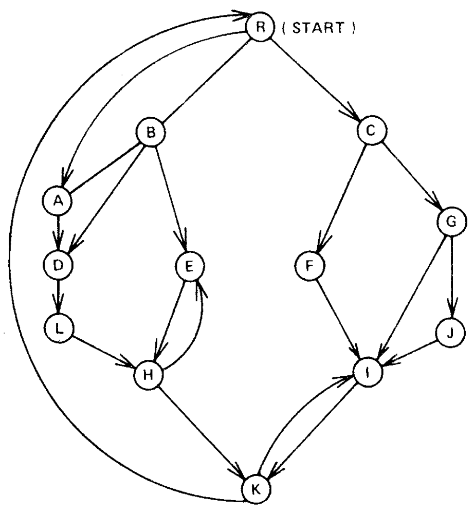
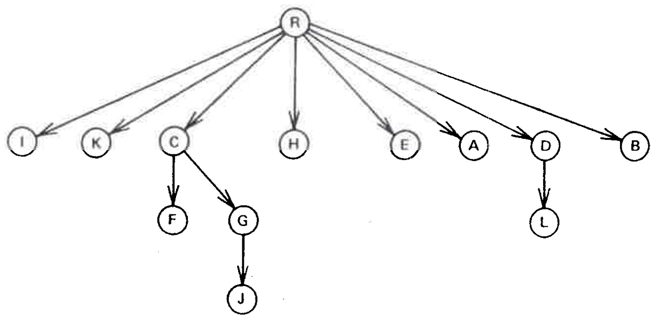
The following graph problem arises in the study of global flow analysis and program optimization [2, 6]. Let \(G=(V,E,r)\) be a flowgraph1 with start vertex \(r\). A vertex \(v\) dominates another vertex \(w \ne v\) in \(G\) if every path from \(r\) to \(w\) contains \(v\). Vertex \(v\) is the immediate dominator of \(w\), denoted \(v = {\it idom}(w)\), if \(v\) dominates \(w\) and every other dominator of \(w\) dominates \(v\).
Theorem 1 [2, 6]. Every vertex of a flowgraph \(G = (V, E, r)\) except \(r\) has a unique immediate dominator. The edges \(\{({\it idom}(w), w) | w \in V - \{r\}\}\) form a directed tree rooted at \(r\), called the dominator tree of \(G\), such that \(v\) dominates \(w\) if and only if \(v\) is a proper ancestor of \(w\) in the dominator tree. See Figures 1 and 2.
We wish to construct the dominator tree of an arbitrary flowgraph \(G\). If \(G\) represents the flow of control of a computer program which we are trying to optimize, then the dominator tree provides information about what kinds of code motion are safe. For further details see [2, 6].
Aho and Ullman [2] and Purdom and Moore [17 (TRANS: 7?)] describe a straightforward algorithm for finding dominators. For each vertex \(v \ne r\), we carry out the following step.
General Step. Determine, by means of a search from \(r\), the set \(S\) of vertices reachable from \(r\) by paths which avoid \(v\). The vertices in \(V - \{v\} - S\) are exactly those which \(v\) dominates.
Knowing the set of vertices dominated by each vertex, it is an easy matter to construct the dominator tree.
To analyze the running time of this algorithm, let us assume that \(G\) has \(m\) edges and \(n\) vertices. Each execution of the general step requires \(O(m)\) time, and the algorithm performs \(n - 1\) executions of the general step; thus the algorithm requires \(O(mn)\) time total.
Aho and Ullman [3] describe another simple algorithm for computing dominators. This algorithm manipulates bit vectors of length \(n\). Each vertex \(v\) has a bit vector which encodes a superset of the dominators of \(v\). The algorithm makes several passes over the graph, updating the bit vectors during each pass, until no further changes to the bit vectors occur. The bit vector for each vertex \(v\) then encodes the dominators of \(v\).
This algorithm requires \(O(m)\) bit vector operations per pass for \(O(n)\) passes, or \(O(nm)\) bit vector operations total. Since each bit vector operation requires \(O(n)\) time, the running time of the algorithm is \(O(n^2m)\). This bound is pessimistic, however; the constant factor associated with the bit vector operations is very small, and on typical graphs representing real programs the number of passes is small (on reducible flowgraphs [3] only two passes are required [4]).
In this paper we shall describe a faster algorithm for solving the dominators problem. The algorithm uses depth-first search [9] in combination with a data structure for evaluating functions defined on paths in trees [14]. We present a simple implementation of the algorithm which runs in \(O(m \log n)\) time and a more sophisticated implementation which runs in \(O(m \alpha(m,n))\) time, where \(\alpha(m,n)\) is a functional inverse of Ackermann's function [1], defined as follows. For integers \(i,j \ge 0\), let \(A(i,0)=0\) if \(i\ge 0\), \(A(0,j)=2^j\) if \(j\ge 1\), \(A(i,1)=A(i-1,2)\) if \(i\ge 1\), and \(A(i,j)=A(i–1,A(i,j-1))\) if \(i\ge 1\), \(j\ge 2\). Then \(\alpha(m,n)\)\(=\min\{i\ge 1\)\(|A(i,\lfloor 2m/n\rfloor)\)\(\gt \log_2 n\}\).
The algorithm is a refinement of earlier versions appearing in [10, 11, 12]. Although proving its correctness and verifying its running time require rather complicated analysis, the algorithm is quite simple to program and is very fast in practice. We programmed both versions of the algorithm in Algol W, a Stanford University version of Algol, and tested the programs on an IBM 370/168. We compared the programs with a transcription into Algol W of the Purdom-Moore algorithm and with an implementation of the bit vector algorithm. On all but the smallest graphs tested our algorithm beat the other methods.
This paper consists of five sections. Section 2 describes the properties of depth-first search used by the algorithm and proves several theorems which imply the correctness of the algorithm. Some knowledge of depth-first search as described in [9] and [10, sec. 2] is useful for understanding this section. Section 3 develops the algorithm, using as primitives two procedures that manipulate trees. Section 4 discusses two implementations, simple and sophisticated, of these tree manipulation primitives. Some knowledge of [14, secs. 1, 2, and 5] is useful for understanding this section. Section 5 presents our experimental results and conclusions.
- 1Appendix A contains the graph-theoretic terminology used in this paper.
2. DEPTH-FIRST SEARCH AND DOMINATORS
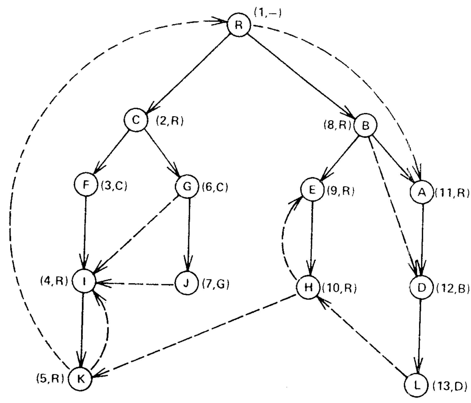
The fast dominators algorithm consists of three parts. First, we perform a depth-first search on the input flowgraph \(G = (V, E, r)\), starting from vertex \(r\), and numbering the vertices of \(G\) from 1 to n in the order they are reached during the search. The search generates a spanning tree \(T\) rooted at \(r\), with vertices numbered in preorder [5]. See Figure 3. For convenience in stating our results, we shall assume in this section that all vertices are identified by number.
The following paths lemma is an important property of depth-first search and is crucial to the correctness of the dominators algorithm.
Lemma 1 [9]. If \(v\) and \(w\) are vertices of \(G\) such that \(v \le w\), then any path from \(v\) to \(w\) must contain a common ancestor of \(v\) and \(w\) in \(T\).
Second, we compute a value for each vertex \(w \ne r\) called its semidominator, denoted by \({\it sdom}(w)\) and defined by \[ \begin{eqnarray} {\it sdom}(w) & = & \min\{v\,|\ \mbox{there is a path $v=v_0,v_1,\ldots,v_k=w$ such that} \nonumber \\ & & \mbox{$u_i\gt w$ for $1 \le i \le k-1$}\} \label{eq1} \end{eqnarray} \] See Figure 3. Third, we use the semidominators to compute the immediate dominators of all vertices.
The semidominators have several properties which make their computation a convenient intermediate step in the dominators calculation. If \(w \ne r\) is any vertex, then \({\it sdom}(w)\) is a proper ancestor of \(w\) in \(T\), and \({\it idom}(w)\) is a (not necessarily proper) ancestor of \({\it sdom}(w)\). If we replace the set of nontree edges of \(G\) by the set of edges \(\{({\it sdom}(w), w)|\mbox{$w\in V$ and $w \ne r$}\}\), then the dominators of vertices in \(G\) are unchanged. Thus if we know the spanning tree and the semidominators, we can compute the dominators.
Lemma 2. For any vertex \(w \ne r\), \({\it idom}(w) \overset{+}{\to} w\)2.
Proof. Any dominator of \(w\) must be on the path in \(T\) from \(r\) to \(w\). ∎
Lemma 3. For any vertex \(w \ne r\), \({\it sdom}(w) \overset{+}{\to} w\).
Proof. Let \({\it parent}(w)\) be the parent of \(w\) in \(T\). Since \(({\it parent}(w),w)\) is an edge of \(G\), by (\(\ref{eq1}\)) \({\it sdom}(w) \le {\it parent}(w) \lt w\). Also by (\(\ref{eq1}\)), there is a path \({\it sdom}(w) = v_0,v_1,\ldots,v_k=w\) such that \(v_i \gt w\) for \(1 \le k \le k-1\). By Lemma 1, some vertex \(v_i\) on the path is a common ancestor of \({\it sdom}(w)\) and \(w\). But such a common ancestor \(v_i\) must satisfy \(v_i \le {\it sdom}(w)\). This means \(i = 0\), i.e. \(v_i = {\it sdom}(w)\), and \({\it sdom}(w)\) is a proper ancestor of \(w\). ∎
Lemma 4. For any vertex \(w\ne r\), \({\it idom}(w) \overset{*}{\to} {\it sdom}(w)\).
Proof. By Lemmas 2 and 3, \({\it idom}(w)\) and \({\it sdom}(w)\) are proper ancestors of \(w\). The path consisting of the tree path from \(r\) to \({\it sdom}(w)\) followed by a path \({\it sdom}(w)=v_0,v_1,\ldots,v_k=w\) such that \(v_i\gt w\) for \(1 \le i \le k-1\) (which must exist by (\(\ref{eq1}\))) avoids all proper descendants of \({\it sdom}(w)\) which are also proper ancestors of \(w\). It follows that \({\it idom}(w)\) is an ancestor of \({\it sdom}(w)\). ∎
Lemma 5. Let vertices \(v\), \(w\) satisfy \(v \overset{*}{\to} w\). Then \(v \overset{*}{\to} {\it idom}(w)\) or \({\it idom}(w) \overset{*}{\to} {\it idom}(v)\).
Proof. Let \(x\) be any proper descendant of \({\it idom}(v)\) which is also a proper ancestor of \(v\). By Theorem 1 and Corollary 1, there is a path from \(r\) to \(v\) which avoids \(x\). By concatenating this path with the tree path from \(v\) to \(w\), we obtain a path from \(r\) to \(w\) wichi avoid \(x\). Thus \({\it idom}(w)\) must be either a descendant of \(v\) or an ancestor of \({\it idom}(v)\). ∎
Using Lemmas 1-5, we obtain two results which provide a way to compute immediate dominators from semidominators.
Theorem 2. Let \(w \ne r\). Suppose every \(u\) for which \({\it sdom}(w)\overset{+}{\to}u\overset{*}{\to}w\) satisfies \({\it sdom}(u)\ge {\it sdom}(w)\). Then \({\it idom}(w)={\it sdom}(w)\).
Proof. By Lemma 4, it suffices to show that \({\it sdom}(w)\) dominates \(w\). Consider any path \(p\) from \(r\) to \(w\). Let \(x\) be the last vertex on this path such that \(x \lt {\it sdom}(w)\). If there is no such \(x\), then \({\it sdom}(w)=r\) dominates \(w\). Otherwise, let \(y\) be the first vertex following \(x\) on the path and satisfying \({\it sdom}(w)\overset{*}{\to}y\overset{*}{\to}w\). Let \(q=(x=v_0,v_1,\ldots,v_k=y)\) be the part of \(p\) from \(x\) to \(y\). We claim \(v_i \lt y\) for \(1\le i\le k-1\). Suppose to the contrary that some \(v_i\) satisfies \(v_i\lt y\). By Lemma 1, some \(v_j\) with \(i\le j\le k-1\) is an ancestor of \(y\). By the choice of \(x\), \(v_j\ge{\it sdom}(w)\), which means \({\it sdom}(w)\overset{*}{\to}v_j\overset{*}{\to}y\overset{*}{\to}w\), contradicting the choice of \(y\). This proves the claim.
The claim together with the definition of semidominators implies that \({\it sdom}(y)\le x\lt {\it sdom}(w)\). By the hypothesis of the theorem, \(y\) cannot be a proper descendant of \({\it sdom}(w)\). Thus \(y={\it sdom}(w)\) and \({\it sdom}(w)\) lies on the path \(p\). Since the path selected was arbitrary, \({\it sdom}(w)\) dominates w. ∎
Theorem 3. Let \(w \ne r\) and let \(u\) be a vertex for which \({\it sdom}(u)\) is minimum among vertices \(u\) satisfying \({\it sdom}(w)\overset{+}{\to}u\overset{*}{\to}w\). Then \({\it sdom}(u)\le{\it sdom}(w)\) and \({\it idom}(u)={\it idom}(w)\).
Proof. Let \(z\) be the vertex such that \({\it sdom}(w)\to z\overset{*}{\to}w\). Then \({\it sdom}(u)\le{\it sdom}(z)\le{\it sdom}(w)\).
By Lemma 4, \({\it idom}(w)\) is an ancestor of \({\it sdom}(w)\) and thus a proper ancestor of \(u\). Thus by Lemma 5 \({\it idom}(w)\overset{*}{\to}{\it idom}(u)\). To prove \({\it idom}(u) ={\it idom}(w)\), it suffices to prove that \({\it idom}(u)\) dominates \(w\).
Consider any path \(p\) from \(r\) to \(w\). Let \(x\) be the last vertex on this path satisfying \(x\lt{\it idom}(u)\). If there is no such \(x\), then \({\it idom}(u)=r\) dominates \(w\). Otherwise, let \(y\) be the first vertex following \(x\) on the path and satisfying \({\it idom}(u)\overset{*}{\to}y\overset{*}{\to}w\). Let \(q=(x=v_0,v_1,v_2,\ldots,v_k=y)\) be the part of \(p\) from \(x\) to \(y\). As in the proof of Theorem 2, the choice of \(x\) and \(y\) implies that \(v_i\gt y\) for \(1\le i\le k-1\). Thus \({\it sdom}(y)\le x\). Since \({\it idom}(u)\le{\it sdom}(u)\) by Lemma 4, we have \({\it sdom}(y)\le x\lt{\it idom}(u)\le{\it sdom}(u)\).
Since \(u\) has the smallest semidominator among vertices on the tree path from \(z\) to \(w\), \(y\) cannot be proper descendant of \({\it sdom}(w)\). Furthermore, \(y\) cannot be both a proper descendant of \({\it idom}(u)\) and an ancestor of \(u\), for if this were the case the path consisting of the tree path from \(r\) to \({\it sdom}(y)\) followed by a path \({\it sdom}(y)=v_0,v_1,\ldots,v_k=y\) such that \(v_i\gt y\) for \(1\le i\le k-1\) followed by the tree path from \(y\) to \(u\) would avoid \({\it idom}(u)\); but no path from \(r\) to \(u\) avoids \({\it idom}(u)\).
Since \({\it idom}(u)\overset{*}{\to}v\overset{+}{\to}u\overset{*}{\to}w\) and \({\it idom}(u)\overset{*}{\to}y\overset{*}{\to}w\), the only remaining possibility is that \({\it idom}(u)=y\). Thus \({\it idom}(u)\) lies on the path from \(r\) to \(w\). Since the path selected was arbitrary, \({\it idom}(u)\) dominates w. ∎
Corollary 1. Let \(w\ne r\) and let \(u\) be a vertex for which \({\it sdom}(u)\) is minimum among vertices \(u\) satisfying \({\it sdom}(w)\overset{+}{\to}u\overset{*}{\to}w\). Then \[ \begin{equation} {\it idom}(w) = \left\{ \begin{array}{ll} {\it sdom}(w) & \mbox{if ${\it sdom}(w)={\it sdom}(u)$} \\ {\it idom}(u) & \mbox{othersize.} \end{array} \right. \label{eq2} \end{equation} \]
Proof. Immediate from Theorems 2 and 3. ∎
The following theorem provides a way to compute semidominators.
Theorem 4. For any vertex \(w\ne r\), \[ {\it sdom}(w) = \min(\{v\,|\,(v,w)\in E \ \mbox{and} \ v \lt w\} \cup \{{\it sdom}(u)\,|\,u\gt w\ \mbox{and} \\ \mbox{there is an edge $(v,w)$ such that $u\overset{*}{\to}v$}\}) \]
Proof. Let \(x\) equal the right-hand side of (\(\ref{eq3}\)). We shall first prove that \({\it sdom}(w)\le x\). Suppose \(x\) is a vertex such that \((x,w)\in E\) and \(x\lt w\). By (\(\ref{eq1}\)), \({\it sdom}(w)\le x\). Suppose on the other hand \(x={\it sdom}(u)\) for some vertex \(u\) such that \(u\gt w\) and there is an edge \((v,w)\) such that \(u\overset{*}{\to}v\). By (\(\ref{eq1}\)) there is a path \(x=v_0,\)\(v_1,\)\(\ldots,\)\(v_j=u\) such that \(v_i\gt u\gt w\) for \(1\ge i\ge j-1\). The tree path \(u=v_j\to v_{j+1}\to\cdots\to v_{k-1}=v\) satisfies \(v_i\ge u\gt w\) for \(j\le i\le k-1\). Thus the path \(x=v_0,\)\(v_1,\)\(\ldots,\)\(v_{k-1}=v\), \(v_k=w\), satisfies \(v_i\gt w\) for \(1\lt i\lt k-1\). By (\(\ref{eq1}\)), \({\it sdom}(w)\le x\).
It remains for us to prove that \({\it sdom}(w)=x\). Let \({\it sdom}(w)=v_0,\)\(v_1,\)\(\ldots,\)\(v_k=w\) be a simple path such that \(v_i\gt w\) for \(1\le i\le k-1\) If \(k=1\), \(({\it sdom}(w), w)\in E\), and \({\it sdom}(w)\lt w\) by Lemma 3. Thus \({\it sdom}(w)\gt x\). Suppose on the other hand that \(k\gt 1\). Let \(j\) be minimum such that \(j\ge 1\) and \(u_j\overset{*}{\to}v_{k-1}\). Such a \(j\) exists since \(k-1\) is a candidate for \(j\).
We claim \(v_i\gt v_j\) for \(1\ge i\ge j-1\). Suppose to the contrary that \(v_i\le v_j\), for some \(i\) in the range \(1\le i\le j-1\), Choose the \(i\) such that \(1\le i\le j-1\) and \(v\), is minimum. By Lemma 1, \(v_i\overset{*}{\to}v_j\), which contradicts the choice of \(j\). This proves the claim.
The claim implies \({\it sdom}(w)={\it sdom}(vj)\ge x\). Thus whether \(k=1\) or \(k\gt 1\), we have \({\it sdom}(w)=x\), and the theorem is true. ∎
- 2Throughout this paper the notation "\(x\overset{*}{\to}y\)" means that \(x\) is an ancestor of \(y\) in the spanning tree \(T\) generated by the depth-first search, and "\(x\overset{+}{\to}y\)" means \(x\overset{*}{\to}y\) and \(x\ne y\).
3. A FAST DOMINATORS ALGORITHM
In this section we develop an algorithm which uses the results in Section 2 to find dominators. Earlier versions of the algorithm appear in [10,11,12]; the version we present is refined to the point where it is as simple to program as the straightforward algorithm [2,7] or the bit vector algorithm [3,4], similar in speed on small graphs, and much faster on large graphs.
The algorithm consists of the following four steps.
Step 1. Carry out a depth-first search of the problem graph. Number the vertices from 1 to n as they are reached during the search. Initialize the variables-used in succeeding steps.
Step 2. Compute the semidominators of all vertices by applying Theorem 4. Carry out the computation vertex by vertex in decreasing order by number.
Step 3. Implicitly define the immediate dominator of each vertex by applying Corollary 1.
Step 4. Explicitly define the immediate dominator of each vertex, carrying out the computation vertex by vertex in increasing order by number.
Our implementation of this algorithm uses the following arrays.
| Input | |
|---|---|
| \({\it succ}(v)\) | The set of vertices w such that (v, w) is an edge of the graph. |
| Computed | |
| \({\it parent}(w)\) | The vertex which is the parent of vertex \(w\) in the spanning tree generated by the search. |
| \({\it pred}(w)\) | The set of vertices v such that \((v,w)\) is an edge of the graph. |
| \({\it semi}(w)\) | A number defined as follows:
|
| \({\it vertex}(i)\) | The vertex whose number is \(i\). |
| \({\it bucket}(w)\) | A set of vertices whose semidominator is \(w\). |
| \({\it dom}(w)\) | A vertex defined as follows:
|
Rather than converting vertex names to numbers during step 1 and converting numbers back to names at the end of the computation, we have chosen to refer to vertices as much as possible by name. Arrays semi and vertex incorporate all that we need to know about vertex numbers. Array semi serves a dual purpose, representing (though not simultaneously) both the number of a vertex and the number of its semidominator. As well as saving storage space, this device allows us to simplify the computation of semidominators by combining the two cases of Theorem 4 into one.
Here is an Algol-like version of step 1.
| 1. | \( {\rm step 1:}\ n := 0 \) | |
| 2. | \( \hspace{30pt}{\bf for} \ {\bf each} \ v \in V \ {\bf do} \ {\it pred}(v) := \emptyset; \ {\it semi}(v) := 0 \ {\bf od}; \) | |
| 3. | \( \hspace{30pt}{\sf DFS}(r); \) | |
Step 1 uses the recursive procedure \({\rm DFS}\), defined below, to carry out the depth-first search. When a vertex \(v\) receives a number \(i\), the procedure assigns \({\it semi}(v):=1\) and \({\it vertex}(i):=v\).
| 1. | \( {\bf procedure} \ {\rm DFS}({\it vertex}): \) | |
| 2. | \( \hspace{12pt}{\bf begin} \) | |
| 3. | \( \hspace{24pt}{\it semi}(v) := n := n + 1; \) | |
| 4. | \( \hspace{24pt}{\it vertex}(n) := v; \) | |
| 5. | \( \hspace{24pt}{\bf comment} \ \mbox{initialize variables for step 2, 3, and 4}; \) | |
| 6. | \( \hspace{24pt}{\bf for \ each} \ w \in {\it succ}(v) \ {\bf do} \) | |
| 7. | \( \hspace{36pt}{\bf if} \ {\it semi}(v) = 0 \ {\bf then} \ {\it parent}(w) := v; {\rm DFS}(u) \ {\bf fi}; \) | |
| 8. | \( \hspace{36pt}{\it add} \ v \ {\it to} \ {\it pred}(w) \ {\bf od} \) | |
| 9. | \( \hspace{12pt}{\bf end} \ {\rm DFS}; \) | |
After carrying out step 1, the algorithm carries out steps 2 and 3 simultaneously, processing the vertices \(w\ne r\) in decreasing order by number. During this computation the algorithm maintains an auxiliary data structure which represents a forest contained in the depth-first spanning tree. More precisely, the forest consists of vertex set \(V\) and edge set \(\{({\it parent}(w), w)|\)vertex \(w\) has been proceessed\(\}\). The algorithm uses one procedure to construct the forest and another to extract information from it:
| \({\rm LINK}(v,w)\) | Add edge \((v,w)\) to the forest. |
| \({\rm EVAL}(v)\) | If \(v\) is the root of a tree in the forest, return \(v\). Otherwise, let \(r\) be the root of the tree in the forest which contains \(v\). Return any vertex \(u\ne r\) of minimum \({\it semi}(u)\) on the path \(r\overset{*}{\to}v\). |
To process a vertex \(w\), the algorithm computes the semidominator applying Theorem of \(w\) by applying Theorem 4. The algorithm assigns \({\it semi}(w):=\min\{{\it semi}({\rm EVAL}(v))|(v,w)\in E\}\). After this assignment, \({\it semi}(w)\) is the number of the semidominator of \(w\). To verify this claim, consider any edge \((v,w)\in E\). If \(v\) is numbered less than \(w\), then \(v\) is unprocessed, which means \(v\) is the root of a tree in the forest and \({\it semi}(v)\) is the number of \(v\). Thus \({\it semi}({\rm EVAL}(v))\) numbered is the number of \(v\). If \(v\) is numbered greater than w, then v has been processed and is not a root. Thus \({\rm EVAL}(v)\) returns a vertex \(u\) among vertices numbered greater than \(w\) satisfying \(u\overset{*}{\to}v\) whose semidominator has the minimum number, and \({\rm semi}({\rm EVAL}(v))\) is the number of \(u\)'s semidominator. This means that the algorithm performs exactly the minimization specified in Theorem 4.
After computing \({\it semi}(w)\), the algorithm adds \(w\) to \({\it bucket}({\it vertex}({\it semi}(w)))\) and adds a new edge to the forest using \({\rm LINK}({\it parent}(w),w)\). This completes step 2 for \(w\). The algorithm then empties \({\it bucket}({\it parent}(w))\), carrying out step 3 for each vertex in the bucket. Let \(v\) be such a vertex. The algorithm implicitly computes the immediate dominator of \(v\) by applying Corollary 1. Let \(u={\rm EVAL}(v)\). Then \(u\) is the vertex satisfying \({\it parent}(w)\overset{+}{\to}u\overset{*}{\to}v\) whose semidominator has minimum number. If \({\it semi(u)={\it semi}(v)\), then \({\it parent}(w)\) is the immediate dominator of \(v\) and the algorithm assigns \({\it dom}(u):={\it parent}(w)\). Otherwise \(u\) and \(v\) have the same dominator and the algorithm assigns \({\it dom}(v)=u\). This completes step 3 for \(v\).
Here is an Algol-like version of steps 2 and 3 which uses \({\rm LINK}\) and \({\rm EVAL}\).
| 1. | \( \hspace{18pt}{\bf comment} \ \mbox{initialize variables} \) | |
| 2. | \( \hspace{18pt}{\bf for} \ i:=n \ {\bf by} \ -1 \ {\bf until} \ 2 \ {\bf do} \) | |
| 3. | \( \hspace{30pt}w := {\it vertex}(i) \) | |
| 4. | \( {\rm step 2:} \ {\bf for \ each} \ v \in {\it pred}(w) \ {\bf do} \) | |
| 5. | \( \hspace{42pt}u := {\rm EVAL}(v); \ {\bf if} \ {\it semi}(u) \lt {\it semi}(w) \ {\bf then} \ {\it semi}(w) := {\it semi}(u) \ {\bf fi \ od}; \) | |
| 6. | \( \hspace{30pt}{\it add} \ w {\it to} \ {\it bucket}({\it vertex}({\it semi}(w))); \) | |
| 7. | \( \hspace{30pt}{\rm LINK}({\it parent}(w),w); \) | |
| 8. | \( {\rm step 3:} \ {\bf for \ each} \ v \in {\it bucket}({\it parent}(w)) \ {\bf do} \) | |
| 9. | \( \hspace{42pt}{\rm delete} \ v \ {\rm from} \ {\it bucket}({\it parent}(w)) \ {\bf do} \) | |
| 10. | \( \hspace{42pt}u := {\rm EVAL}(u); \) | |
| 11. | \( \hspace{42pt}{\it dom}(v) := {\bf if} \ {\it semi}(u) \lt {\it semi}(u) \ {\bf then} \ u \) | |
| 12. | \( \hspace{90pt}{\bf else} \ {\it parent}(w) \ {\bf fi \ od \ od}; \) | |
Step 4 examines vertices in increasing order by number, filling in the immediate dominators not explicitly computed by step 3. Here is an Algol-like version of step 4.
| 1. | \( {\rm step 4:} \ {\bf for} \ i:=2 \ {\bf until} \ n \ {\bf do} \) | |
| 2. | \( \hspace{42pt}w := {\it vertex}(i); \) | |
| 3. | \( \hspace{42pt}{\bf if} \ {\it dom}(w)\ne {\it vertex}({\it semi}(w)) \ {\bf then} \ {\it dom}(w) := {\it dom}({\it dom}(w)) \ {\bf fi \ od}; \) | |
| 4. | \( \hspace{30pt}{\it dom}(r) := 0 \) | |
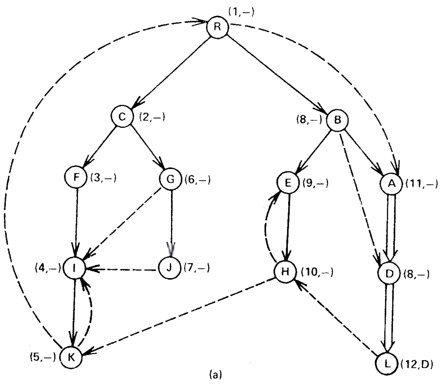
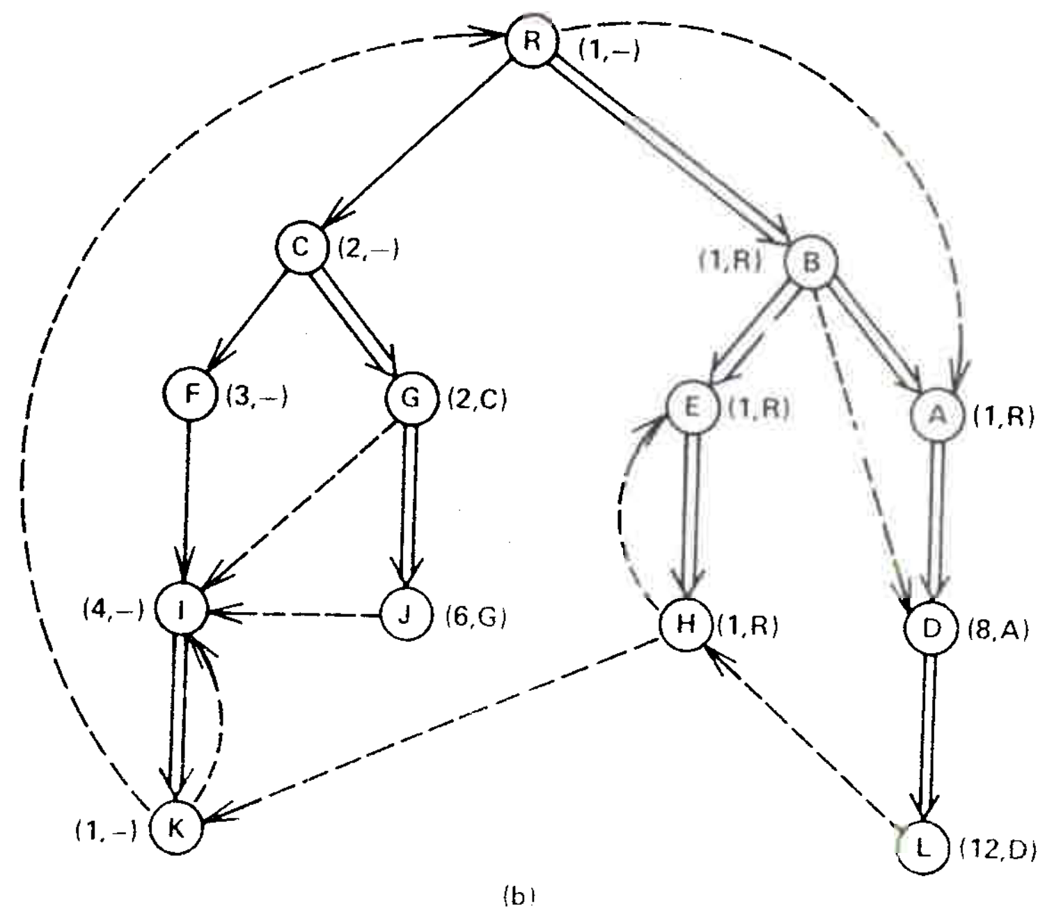
This completes our presentation of the algorithm except for the implementation of \({\rm LINK}\) and \({\rm EVAL}\). Figure 4 illustrates how the algorithm works.
Fig. 1(a) is a snapshot of the graph just before vertex A is processed. Two edges \((B A)\) and \((R,A)\) enter vertex \(A\), giving 8 (the number of \(B\)) and 1 (the number of \(R\)) as candidates for \({\it semi}(A)\). The algorithm assigns \({\it semi}(A):=1\), places \(A\) in \({\it bucket}(R)\), and adds edge \((B,A)\) to the forest. Then the algorithm empties \({\it bucket}(B)\), which contains only \(D\). \({\rm EVAL}(D)\) produces \(A\) as the vertex on the path \(B\overset{+}{\to}A\overset{*}{\to}D\) with minimum \({\it semi}\). Since \({\it semi}(A)=1\lt 8={\it semi}(D),\) \({\it idom}(A)={\it idom}(D)\) and the algorithm assigns \({\rm dom}(D)=A\).
Figure 4(b) is a snapshot of the graph just before vertex \(I\) is processed. Four edges \((F,I)\), \((G,I)\), \((J,I)\), and \((K,I)\) enter vertex \(I\), giving 3 (the number of \(F\)), 2 (\({\it semi}(G)\)), 2 (\({\it semi}(G)\)), and 1 (\({\it semi}(K)\)), respectively, as candidates for \({\it semi}(I)\). The algorithm assigns \({\it semi}(I)=1\), places \(I\) in \({\it bucket}(R)\), and adds edge \((F,I)\) to the forest. Then the algorithm empties \({\it bucket}(F)\), which contains nothing.
Appendix B contains a complete Algol-like version of the algorithm, including variable declarations and initialization. Using Theorem 4 and Corollary 1, it is not hard to prove that after execution of the algorithm, \({\it dom}(v)={\it idom}(v)\) for each vertex \(v\ne r\), assuming that \({\rm LINK}\) and \({\rm EVAL}\) perform as claimed. The running time of the algorithm is \(O(m+n)\) plus time for \(n-1\) \({\rm LINK}\) and \(m+n-1\) \({\rm EVAL}\) instructions.
4. IMPLEMENTATION OF LINK AND EVAL
Two ways to implement \({\rm LINK}\) and \({\rm EVAL}\), one simple and one sophisticated, are provided in [14]. We shall not discuss the details of these methods here, but merely provide Algol-like implementations of \({\rm LINK}\) and \({\rm EVAL}\) which are adapted from [14].
The simple method uses path compression to carry out \({\rm EVAL}\). To represent the forest built by the \({\rm LINK}\) instructions (henceforth called the \({\it forest}\)), the algorithm uses two arrays, \({\it ancestor}\) and \({\it label}\). Initially \({\it ancestor}(v)=0\) and \({\it label}(v)=v\) for each vertex \(v\). In general \({\it ancestor}(v)=0\) only if \(v\) is a tree root in the forest; otherwise \({\it ancestor}(v)\) is an ancestor of \(v\) in the forest.
The algorithm maintains the labels so that they satisfy the following property. Let \(v\) be any vertex, let \(r\) be the root of the tree in the forest containing \(v\), and let \(v=v_k,v_{k-1},\ldots,v_0=r\) be such that \({\rm ancestor}(v_i)=v_{i-1}\) for \(1\le i\le i\). Let \(x\) be a vertex such that \({\it semi}(x)\) is minimum among vertices \(x\in\{{\it label}(v_i)|1\le i\le k\}\). Then \[ \begin{equation} \mbox{$x$ is a vertex such that ${\it semi}(x)$ is minimum among vertices $x$} \\ \mbox{satisfying $r \overset{+}{\to} x \overset{*}{\to} v$.} \label{eq3} \end{equation} \]
To carry out \({\rm LINK}(v,w)\), the algorithm assigns \({\it ancestor}(w):=v\). To carry out \({\rm EVAL}(v)\), the algorithm follows ancestor pointers to determine the sequence \(v=v_k,v_{k-1},\ldots,v_0=r\) such that \({\it ancestor}(v_i)=v_{i-1}\) for \(1\le i\le k\). If \(v=r\), \(v\) is returned. Otherwise, the algorithm performs a path compression by assigning \({\it ancestor}(v_i):=r\) for \(i\) from 2 to \(k\), simultaneously updating labels to maintain (\(\ref{eq3}\)) as follows: If \({\it semi}({\it label}(v_{i-1}))\lt {\it semi}({\it label}(v_i))\), then \({\it label}(v_i):={\it label}(v_{i-1})\). Then \({\it label}(v)\) is returned. Here is an Algol-like procedure for \({\rm EVA}\)L.
| 1. | \( {\bf vertex \ procedure} \ {\rm EVAL}(v); \) | |
| 2. | \( \hspace{12pt}{\bf if} \ {\it ancestor}(v) = 0 \ {\bf then} \ {\rm EVAL} := v \) | |
| 3. | \( \hspace{12pt}{\bf else} \ {\rm COMPRESS}(v); {\rm EVAL} := {\it label}(v) \ {\bf fi}; \) | |
Recursive procedure \({\rm COMPRESS}\), which carries out the path compression, is defined by
| 1. | \( {\bf procedure} \ {\rm COMPRESS}(v); \) | |
| 2. | \( \hspace{12pt}{\bf comment} \ \mbox{this procedure assumes ${\it ancestor}(v)\ne 0$}; \) | |
| 3. | \( \hspace{12pt}{\bf if} \ {\it ancestor}({\it ancestor}(v)) \ne 0 \ {\bf then} \) | |
| 4. | \( \hspace{24pt}{\rm COMPRESS}({\it ancestor}(v)); \) | |
| 5. | \( \hspace{24pt}{\bf if} \ {\it semi}({\it label}({\it ancestor}(v))) \lt {\it semi}({\it label}(v)) \ {\bf then} \) | |
| 6. | \( \hspace{36pt}{\it label}(v) := {\it label}({\it ancestor}(v)) \ {\bf fi}; \) | |
| 7. | \( \hspace{24pt}{\it ancestor}(v) := {\it ancestor}({\it ancestor}(v)) \ {\bf fi}; \) | |
The time required for \(n-1\) \({\rm LINK}\)s and \(m+n-1\) \({\rm EVAL}\)s using this implementation is \(O(m \log n)\) [14]. Thus the simple version of the dominators algorithm requires \(O(m \log n)\) time.
The sophisticated method uses path compression to carry out the \({\rm EVAL}\) instructions but implements the \({\rm LINK}\) instruction so that path compression is carried out only on balanced trees. See [14]. The sophisticated method requires two additional arrays, \({\it size}\) and \({\it child}\). Initially \({\it size}(v)=1\) and \({\it child}(v)=0\) for all vertices \(v\). Here are Algol-like implementations of \({\rm EVAL}\) and \({\rm LINK}\) using the sophisticated method. These procedures are adapted from [14].
| 1. | \( {\bf vertex \ procedure} \ {\rm EVAL}(v); \) | |
| 2. | \( \hspace{12pt}{\bf comment} \ \mbox{procedure ${\rm COMPRESS}$ used here is identical to that in the simple method.} \) | |
| 3. | \( \hspace{12pt}{\bf if} \ {\it ancestor}(v)=0 \ {\bf then} \ {\rm EVAL} := {\it label}(v) \) | |
| 4. | \( \hspace{12pt}{\bf else} \ {\rm COMPRESS}(v); \) | |
| 5. | \( \hspace{24pt}{\rm EVAL} := {\bf if} \ {\it semi}({\it label}({\it ancestor}(v))) \ge {\it semi}({\it label}(v)) \) | |
| 6. | \( \hspace{66pt}{\bf then} \ {\it label}(v) \ {\bf else} \ {\it label}({\it ancestor}(v)) \ {\bf fi \ fi}; \) | |
| 7. | \( {\bf procedure} \ {\rm LINK}(v,w); \) | |
| 8. | \( \hspace{12pt}{\bf begin} \) | |
| 9. | \( \hspace{24pt}{\bf comment} \ \mbox{this procedure assumes for convenience that ${\it size}(0)={\it label}(0)={\it semi}(0)=0$}; \) | |
| 10. | \( \hspace{24pt}s := w \) | |
| 11. | \( \hspace{24pt}{\bf while} \ {\it semi}({\it label}(w)) \lt {\it semi}({\it label}({\it child}(s))) \ {\bf do} \) | |
| 12. | \( \hspace{36pt}{\bf if} \ {\it size}(s) + {\it size}({\it child}({\it child}(s))) \ge 2* {\it size}({\it child}(s)) \ {\bf then} \) | |
| 13. | \( \hspace{48pt}{\it parent}({\it child}(s)) := s; \ {\it child}(s) := {\it child}({\it child}(s)) \) | |
| 14. | \( \hspace{36pt}{\bf else} \ {\it size}({\it child}(s)) := {\it size}(s); \) | |
| 15. | \( \hspace{48pt}s := {\it parent}(s) := {\it child}(s) \ {\bf fi \ od}; \) | |
| 16. | \( \hspace{24pt}{\it label}(s) := {\it label}(w); \) | |
| 17. | \( \hspace{24pt}{\it size}(v) := {\it size}(v) + {\it size}(w); \) | |
| 18. | \( \hspace{24pt}{\bf if} \ {\it size}(v) \lt 2 * {\it size}(w) \ {\bf then} \ s, {\it child}(v) := {\it child}(v), s \ {\bf fi}; \) | |
| 19. | \( \hspace{24pt}{\bf while} \ s \ne 0 \ {\bf do} \ {\it parent}(s) := v;\ s := {\it child}(s) \ {\bf od} \) | |
| 20. | \( \hspace{12pt}{\bf end} \ {\rm LINK} \) | |
With this implementation, the time required for \(n-1\) \({\rm LINK}\)s and \(m+n-1\) \({\rm EVAL}\)s is \(O(m\alpha(m,n))\), where \(\alpha\) is the functional inverse of Ackerman's function [1] defined in the Introduction. Thus the sophisticated version of the dominators algorithm requires \(O(m\alpha(m,n))\) time.
5. EXPERIMENTAL RESULTS AND CONCLUSIONS
We performed extensive experiments in order to qualitatively compare the actual performance of our algorithm with that of the Purdom-Moore algorithm [7] and that of the bit vector algorithm. We translated both versions of our algorithm as contained in Appendix B into Algol W and ran the programs on a series of randomly generated program flowgraphs.
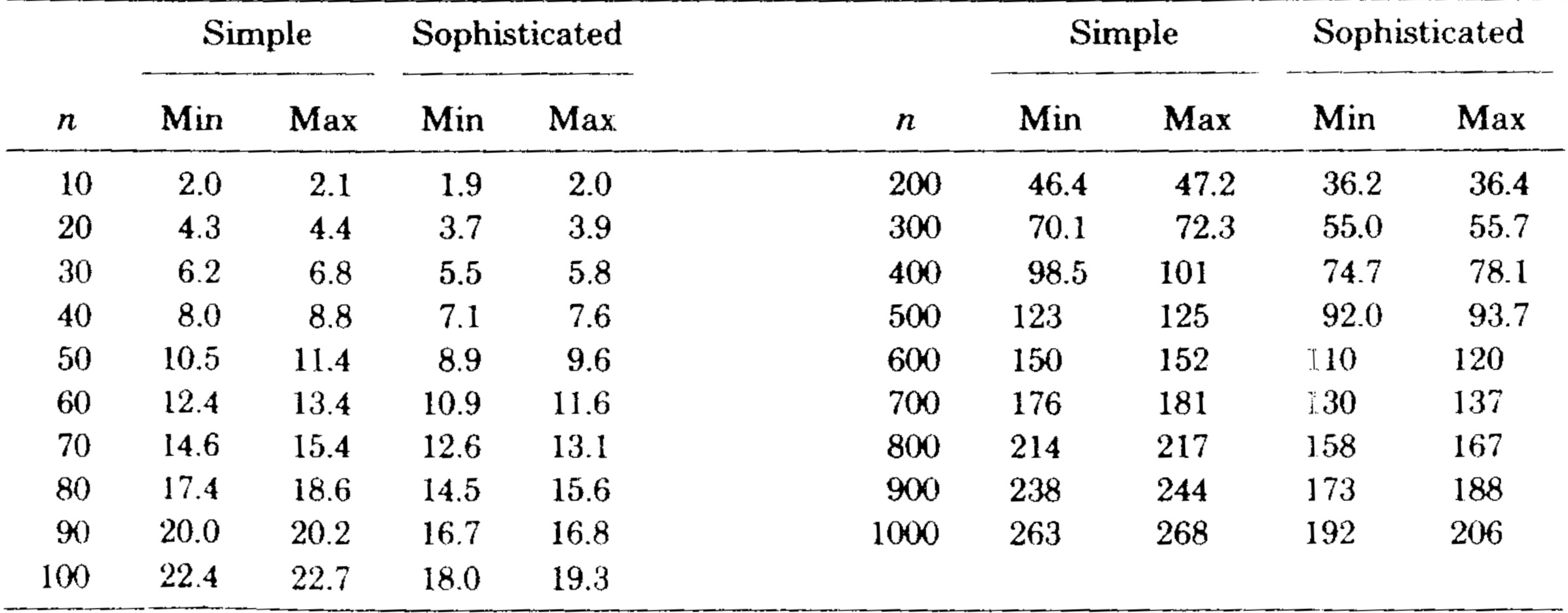
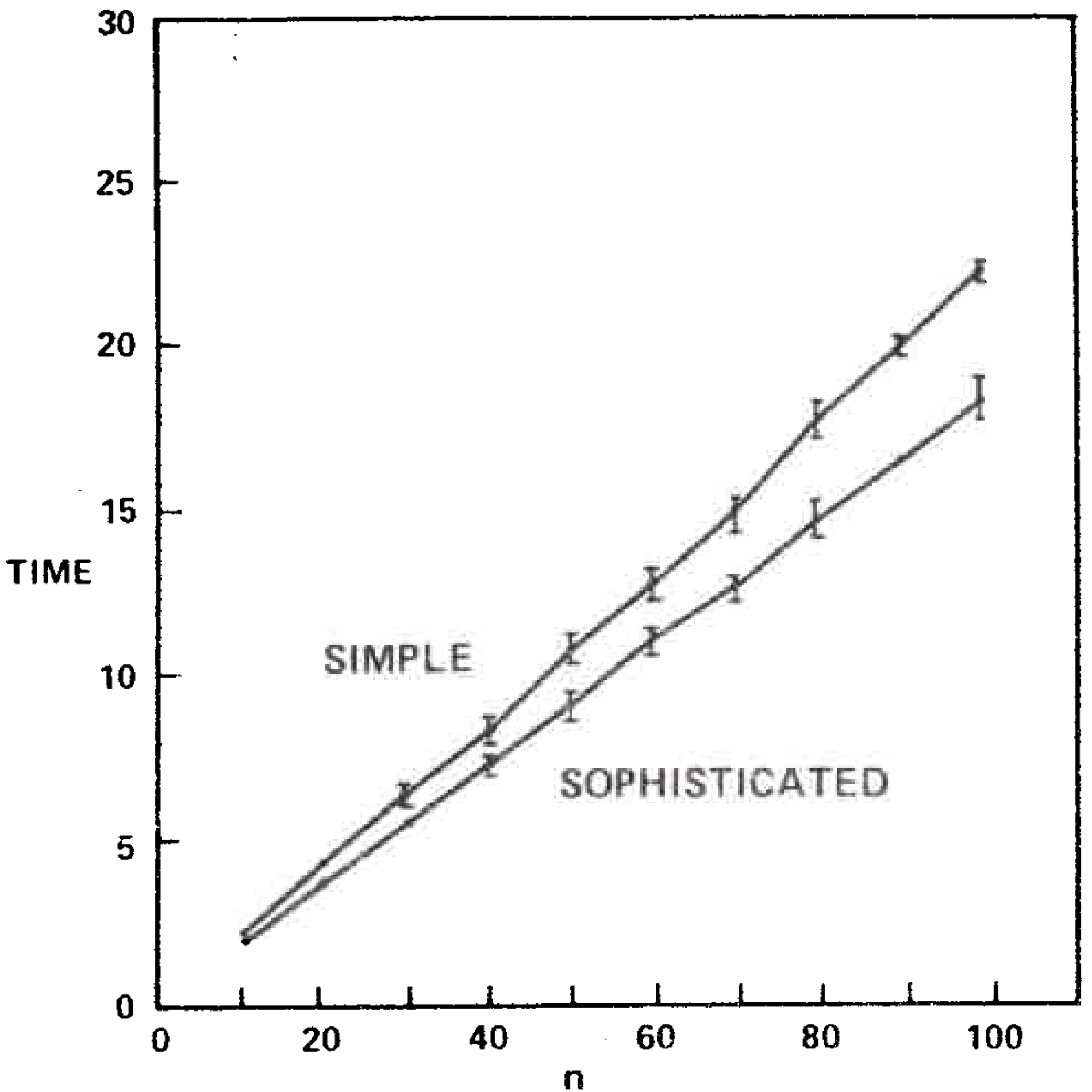
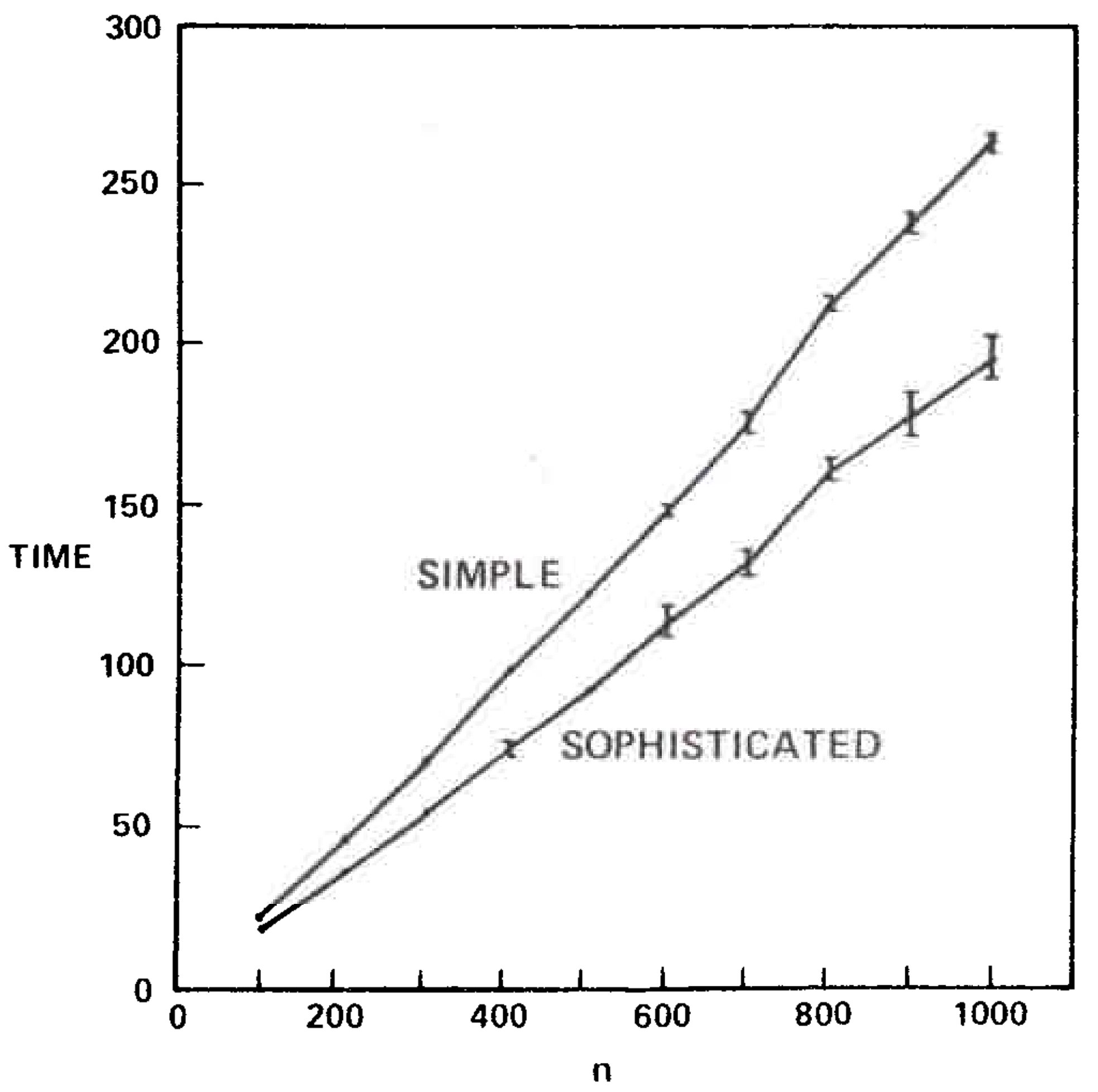
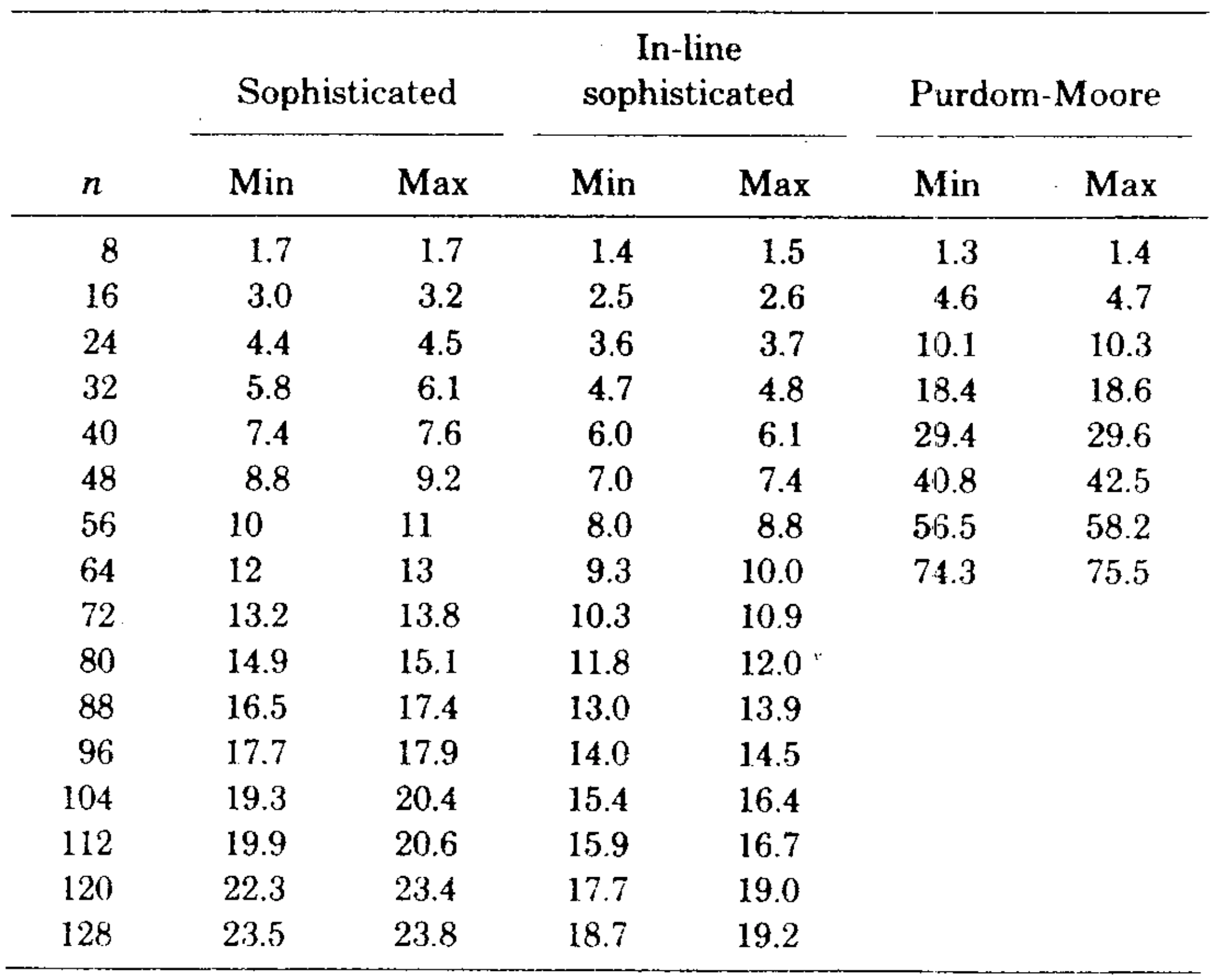
Table 1 and Figures 5 and 6 illustrate the results. The sophisticated version beat the simple version on all graphs tested. The relative difference in speed was between 5 and 25 percent increasing with increasing \(n\). It is important to note that the running times of the algorithms are insensitive to the way the test graphs are selected; for fixed \(m\) and \(n\) the running times vary very little on different graphs, whether the graphs are chosen randomly or by some other method. This is also true for the Purdom-Moore algorithm.
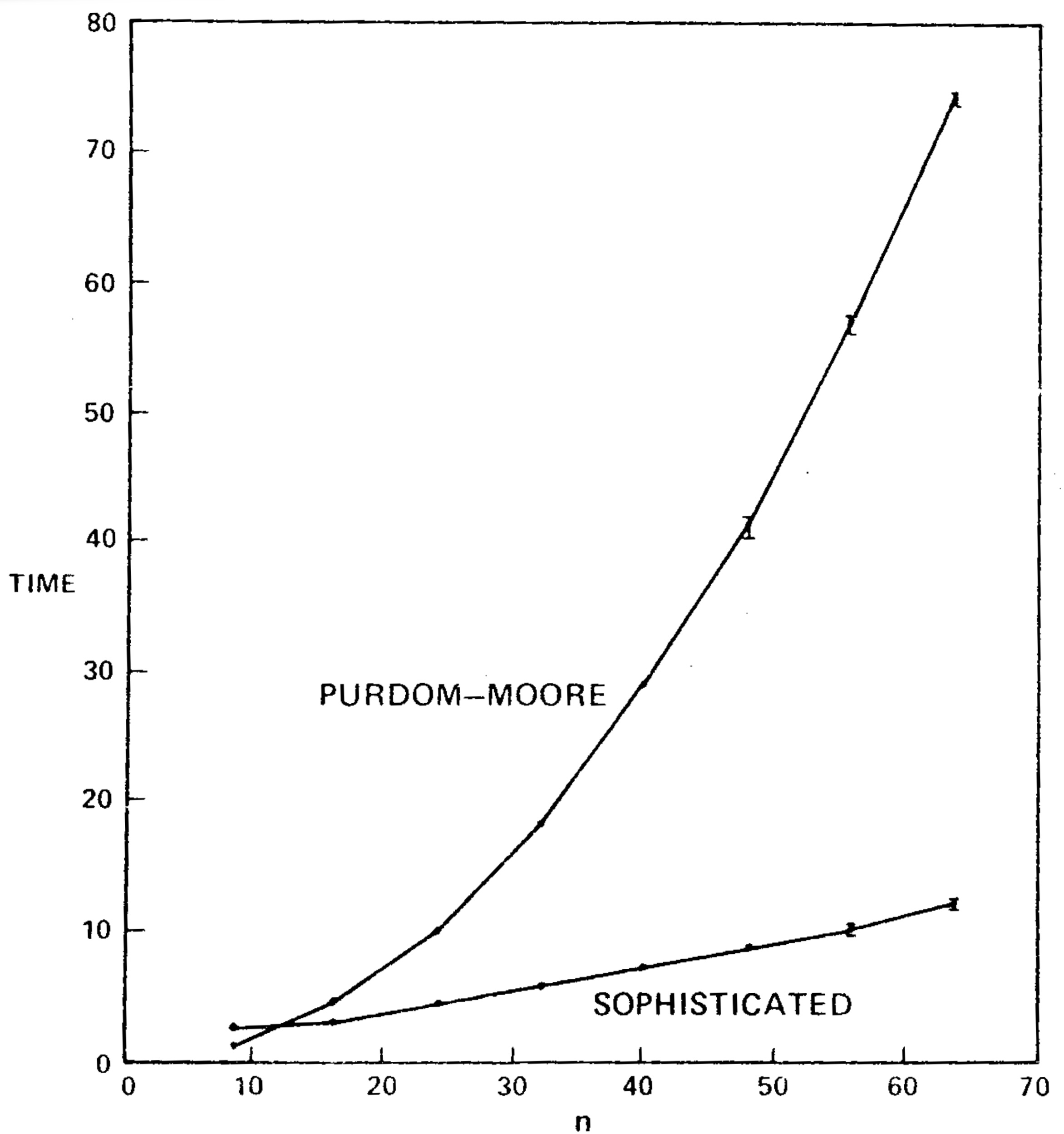
We transcribed the Purdom-Moore algorithm into Algol W and ran it and the sophisticated version of our algorithm on another series of program flowgraphs. Table II and Figure 7 show the results. Our algorithm was faster on all graphs tested except those with \(n=8\). The Purdom-Moore algorithm rapidly became noncompetitive as n increased. The tradeoff point was about \(n=10\).
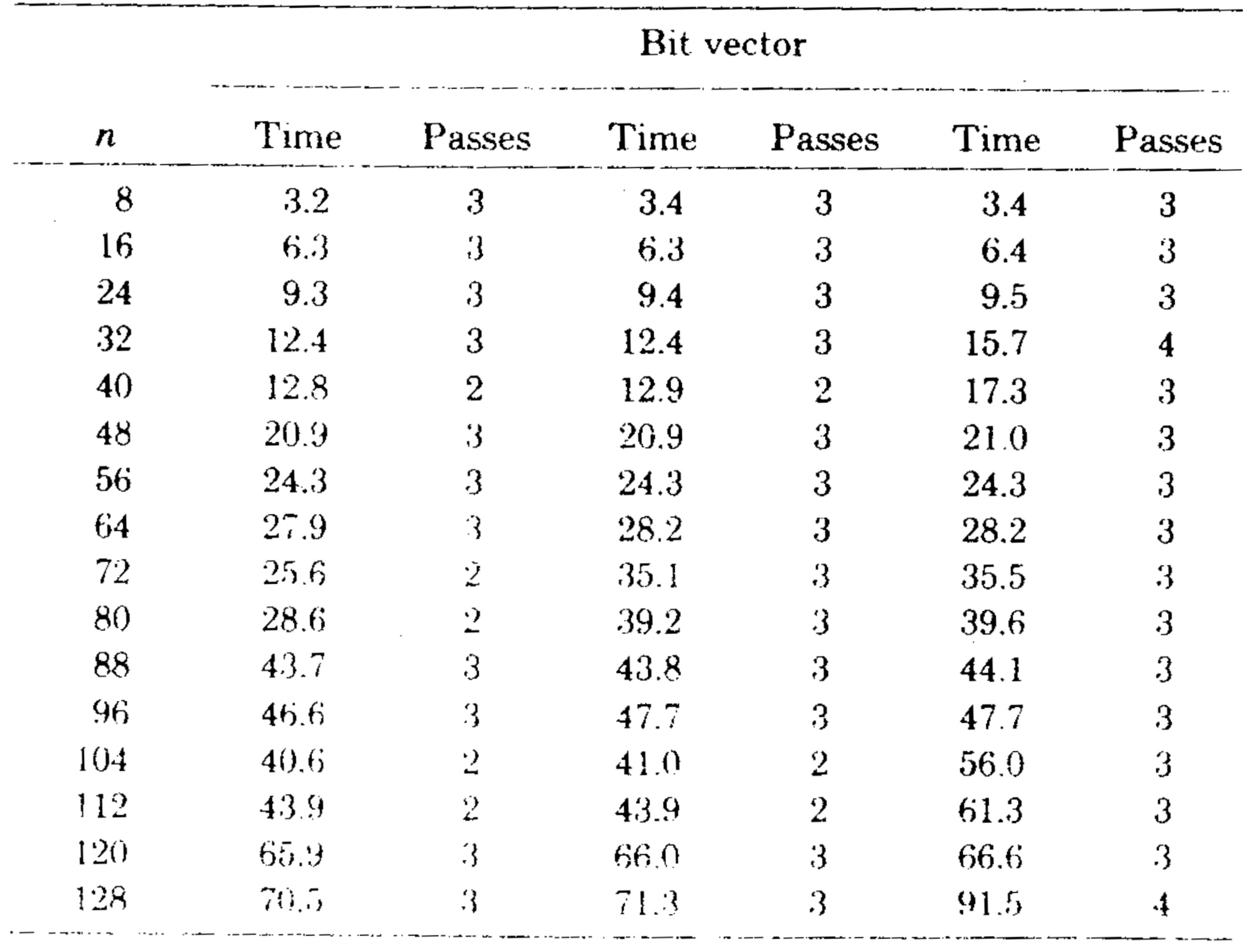
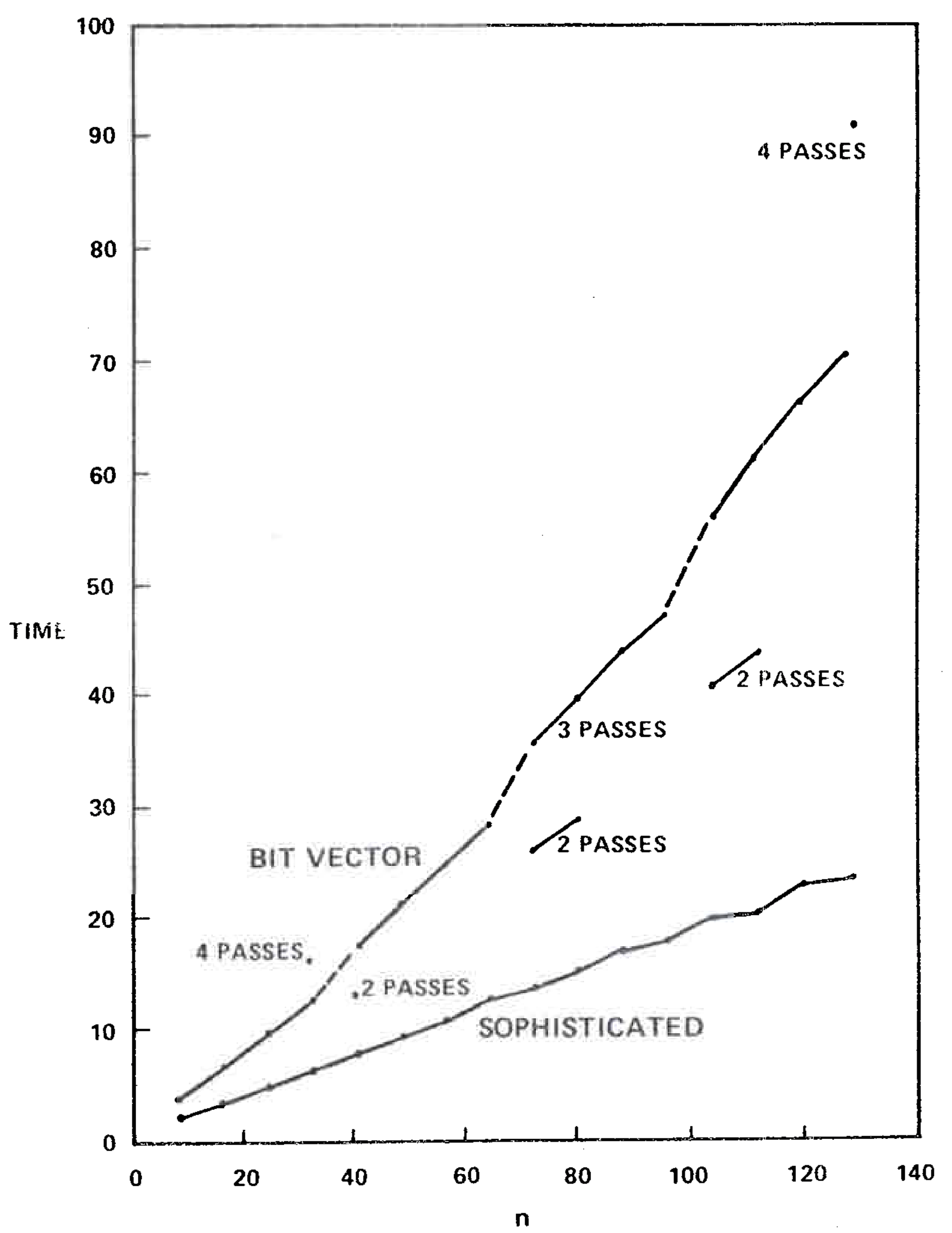
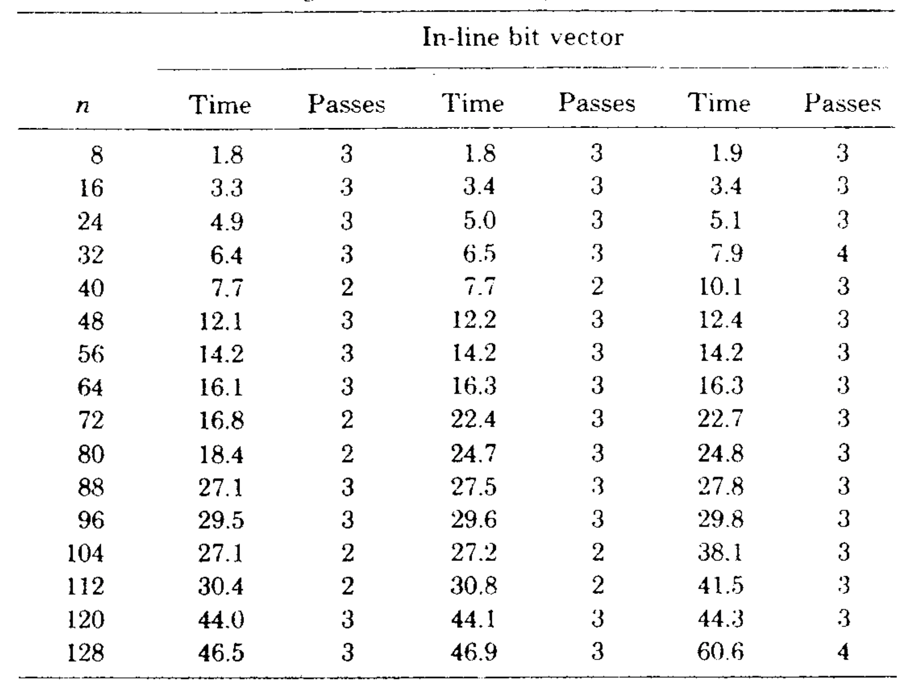
We implemented the bit vector algorithm using a set of procedures for manipulating multiprecision bit vectors. (Algol W allows bit vectors only of length 32 or less.) Table III gives the running time of this algorithm on the second series of test graphs, and Figure 8 compares the running times of the bit vector algorithm and the sophisticated version of our algorithm. The speed of the bit vector algorithm varied not only with \(m\) and \(n\), but also with the number of passes required (two, three, or four on our test graphs). However, the bit vector method was always slower than our algorithm.
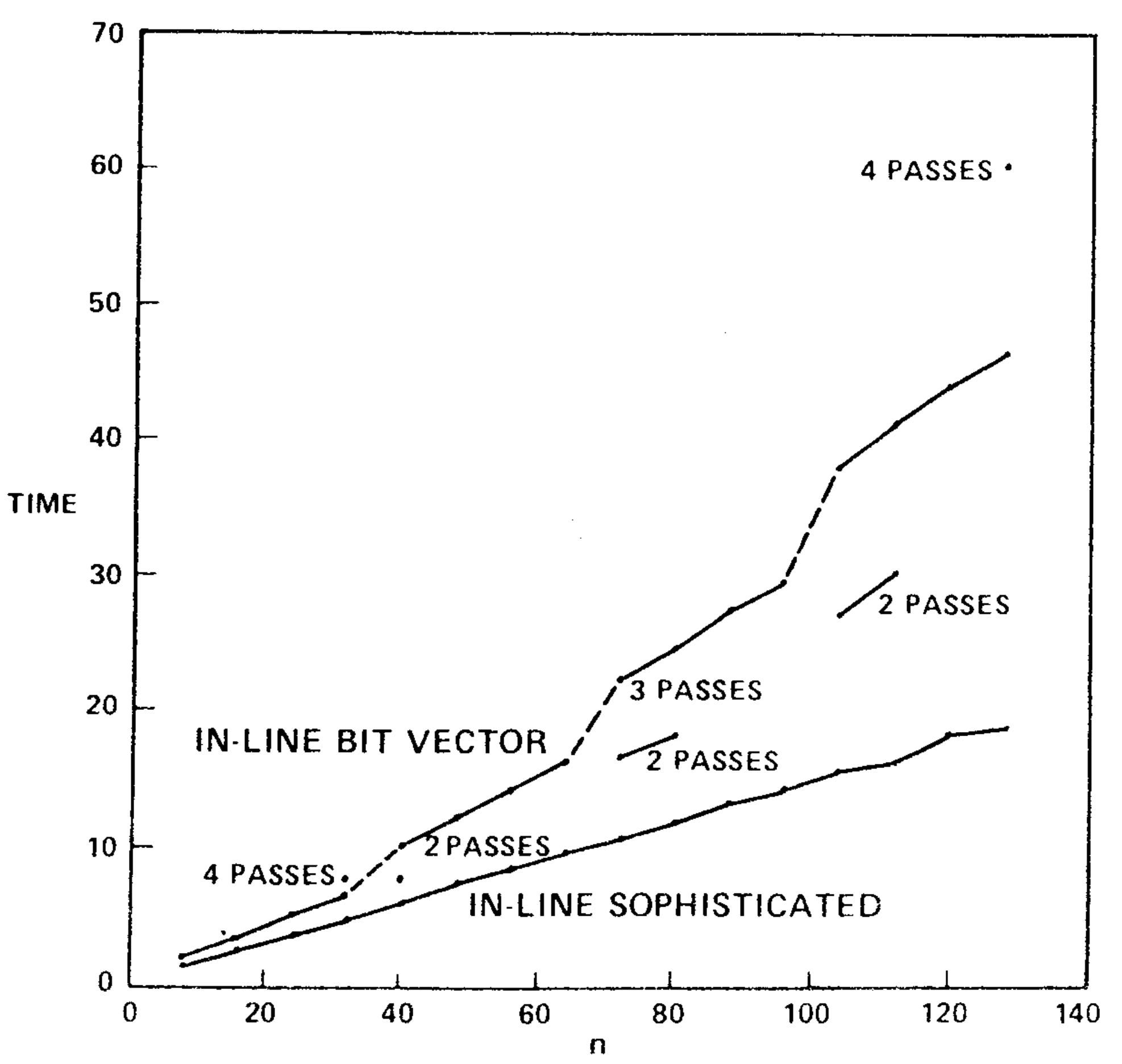
There are several ways in which the bit vector algorithm can be made more competitive. First, the bit vector procedures can be inserted in-line to save the overhead of procedure calls. We made this change and observed a 33-45-percent speedup. The corresponding change in the fast algorithm, inserting \({\rm LINK}\) and \({\rm EVAL}\) in-line, produced a 20-percent speedup. These changes made the bit vector algorithm almost as fast as our algorithm on graphs of less than 32 vertices, but on larger graphs the bit vector algorithm remained substantially slower than our algorithm. See Tables I and IV and Figure 9.
Second, the bit vector procedures can be written in assembly language. To provide a fair comparison with the fast algorithm, it would be necessary to write \({\rm LINK}\) and \({\rm EVAL}\) in assembly language. We did not try this approach, but we believe that the fast algorithm would still beat the bit vector algorithm on graphs of moderate size.
Third, use of the bit vector algorithm can be restricted to graphs known to be reducible. On a reducible graph only one pass of the bit vector algorithm is necessary, because the only purpose served by the second pass is to prove that the bit vectors do not change, a fact guaranteed by the reducibility of the graph. We believe that a one-pass in-line bit vector algorithm would be competitive with the fast algorithm on reducible graphs of moderate size, but only if one ignores the time needed to test reducibility.
The bit vector algorithm has two disadvantages not possessed by the fast algorithm. First, it requires \(O(n^2)\) storage, which may be prohibitive for large values of \(n\). Second, the dominator tree, not the dominator relation, is required for many kinds of global flow analysis [8,13], but the bit vector algorithm computes only the dominator relation. Computing the relation from the tree is easy, requiring constant time per element of the relation or \(O(n)\) bit vector operations total. However, computing the tree from bit vectors encoding the relation requires \(O(n^2)\) time in the worst case.
We can summarize the good and bad points of the three algorithms as follows: The Purdom-Moore algorithm is easy to explain and easy to program but slow on all but small graphs. The bit vector algorithm is equally easy to explain and program, faster than the Purdom-Moore algorithm, but not competitive in speed with the fast algorithm unless it is run on small graphs which are reducible or almost reducible. The fast algorithm is much harder to prove correct but almost as easy to program as the other two algorithms, is competitive in speed on small graphs, and is much faster on large graphs. We favor some version of the fast algorithm for practical applications.
We conclude with a few comments on ways to improve the efficiency of the fast algorithm. One can speed up the algorithm by rewriting \({\rm DFS}\) and \({\rm COMPRESS}\) as nonrecursive procedures which use explicit stacks. One can avoid using an auxiliary stack for \({\rm COMPRESS}\) by instead using a trick of reversing ancestor pointers; see [12]. A similar trick allows one to avoid the use of an auxiliary stack for \({\rm DFS}\). One can Save some additional storage by combining certain arrays, such as parent and ancestor. These modifications save running time and storage space, but only at the expense of program clarity.
APPENDIX A. GRAPH-THEORETIC TERMINOLOGY
...
APPENDIX B. THE COMPLETE DOMINATORS ALGORITHM
...
REFERENCES
- ACKERMANN, W. Zum Hildertschen Aufbau der reellen Zahlen. Math. Ann. 99 (1928), 118-133.
- AHO, A.V., And Ullman, J.D. The Theory of Parsing, Translation, and Compiling, Vol. II: Compiling. Prentice-Hall, Englewood Cliffs, N.J., 1972.
- AHO, A.V., And Ullman, J.D. Principles of Compiler Design. Addison-Wesley, Reading, Mass., 1977.
- HECHT, M.S., AND ULLMAN, J.D. A simple algorithm for global data flow analysis problems. SIAM J. Comput. 4 (1973), 519-532.
- KNUTH, D.E. The Art of Computer Programming, Vol. 1: Fundamental Algorithms. Addison-Wesley, Reading, Mass., 1968.
- LORRY, E.S., AND Medlock, C.W. Object code optimization. Comm. ACM 12, 1 (Jan. 1969), 13–22.
- PURDOM, P.W., AND MOORE, E.F. Algorithm 430: Immediate predominators in a directed graph. Comm. ACM 15, 8 (Aug. 1972), 777-778.
- REIF, J. Combinatorial aspects of symbolic program analysis. Tech. Rep. TR-11-77, Center for Research in Computing Technology, Harvard U., Cambridge, Mass., 1977.
- TARJAN, R.E. Depth-first search and linear graph algorithms. SIAM J. Comptng. 1 (1972), 146-160.
- TARJAN, R. Finding dominators in directed graphs SIAM J. Comptng. 3 (1974), 62-89.
- TARJAN, R.E. Edge-disjoint spanning trees, dominators, and depth-first search. Tech. Rep. STAN-CS-74-455, Comptr. Sci. Dept., Stanford U., Stanford, Calif., 1974.
- TARJAN, R.E. Applications of path compression on balanced trees. Tech. Rep. STAN-CS-75-512. Comptr. Sci. Dept., Stanford U., Stanford, Calif., 1975.
- TARJAN, R.E. Solving path problems on directed graphs. Tech. Rep. STAN-CS-528, Comptr. Sci. Dept., Stanford U., Stanford, Calif., 1975.
- TARJAN, R.E. Applications of path compression on balanced trees. To appear in J. ACM.
Transcription Note
A 1979 paper on dominator tree. A transcription of an old PDF for the purpose of reading it in machine translation.
- LENGAUER, Thomas; TARJAN, Robert Endre. A fast algorithm for finding dominators in a flowgraph. ACM Transactions on Programming Languages and Systems (TOPLAS), 1979, 1.1: 121-141.