
Slate: Stratified Hash Tree
This is an AI-translated content from Japanese version.
 Preface
We propose Slate, a Stratified Hash Tree, which is a hash tree structure that is efficient for appends and access with respect to real-world memory hierarchy, and retains a complete history of cumulative structural changes. The core requirements in the design of this data structure are the following three points:
Based on the principle of temporal locality, it must have a structure that makes I/O operations on recently accessed data efficient.
It must be able to compare multiple data streams, such as transaction logs in a distributed environment, and quickly identify their differences and divergence points.
As a persistent data structure, it must maintain all past versions.
The essence of this structure is an appendable hash tree (Merkle tree), and like a general hash tree, it can be used to verify data corruption or tampering using small data fragments.
The content of this document is currently personal research, as I could not find any papers or books on the corresponding algorithm. I have named this structure the Stratified Hash Tree because of its structural feature of growing in layers of nodes as elements are added.

For a concrete implementation, please refer to https://github.com/torao/stratified-hash-tree.
Table of Contents
- Preface
- Abstract
- 1 Introduction
- 2 Related Work
- 3 Preliminaries and Definitions
- 4 The Slate Data Structure
- 5 Operations and Algorithms
- 6 Complexity Analysis
- 7 Implementation Considerations
- 8 Applications
- 9 Experimental Evaluation
- 10 Discussion
- 11 Conclusion
- References
Abstract
1 Introduction
A Stratified Hash Tree (Slate) is a partially persistent data structure hash tree (Merkle tree) with an append-efficient structure. It is suitable for list structures that link verifiable data, such as transaction logs or blockchains, identified by a single incrementally increasing number \(i\), for purposes like tamper detection or fork detection. The serialization format of this data structure is very simple and can be efficiently represented in a file (block device) on secondary storage like an SSD. The data append operation is very fast as it is completed only by appending to the file.
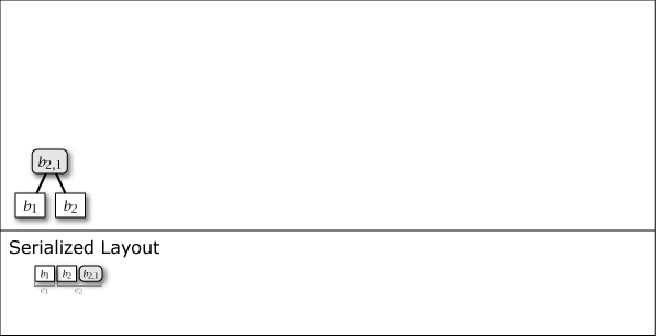
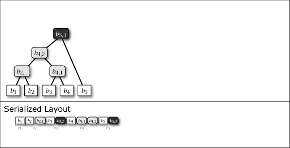
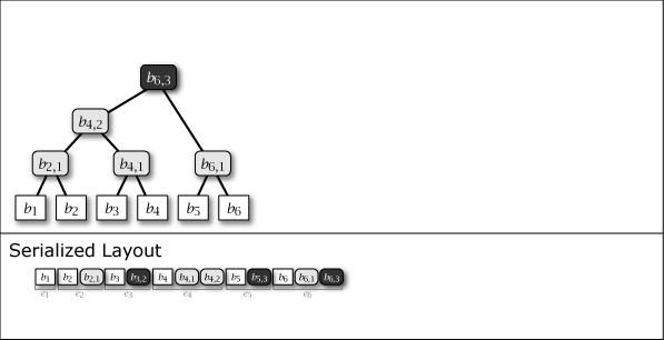
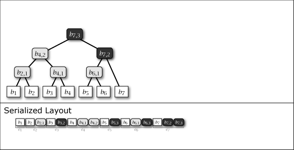
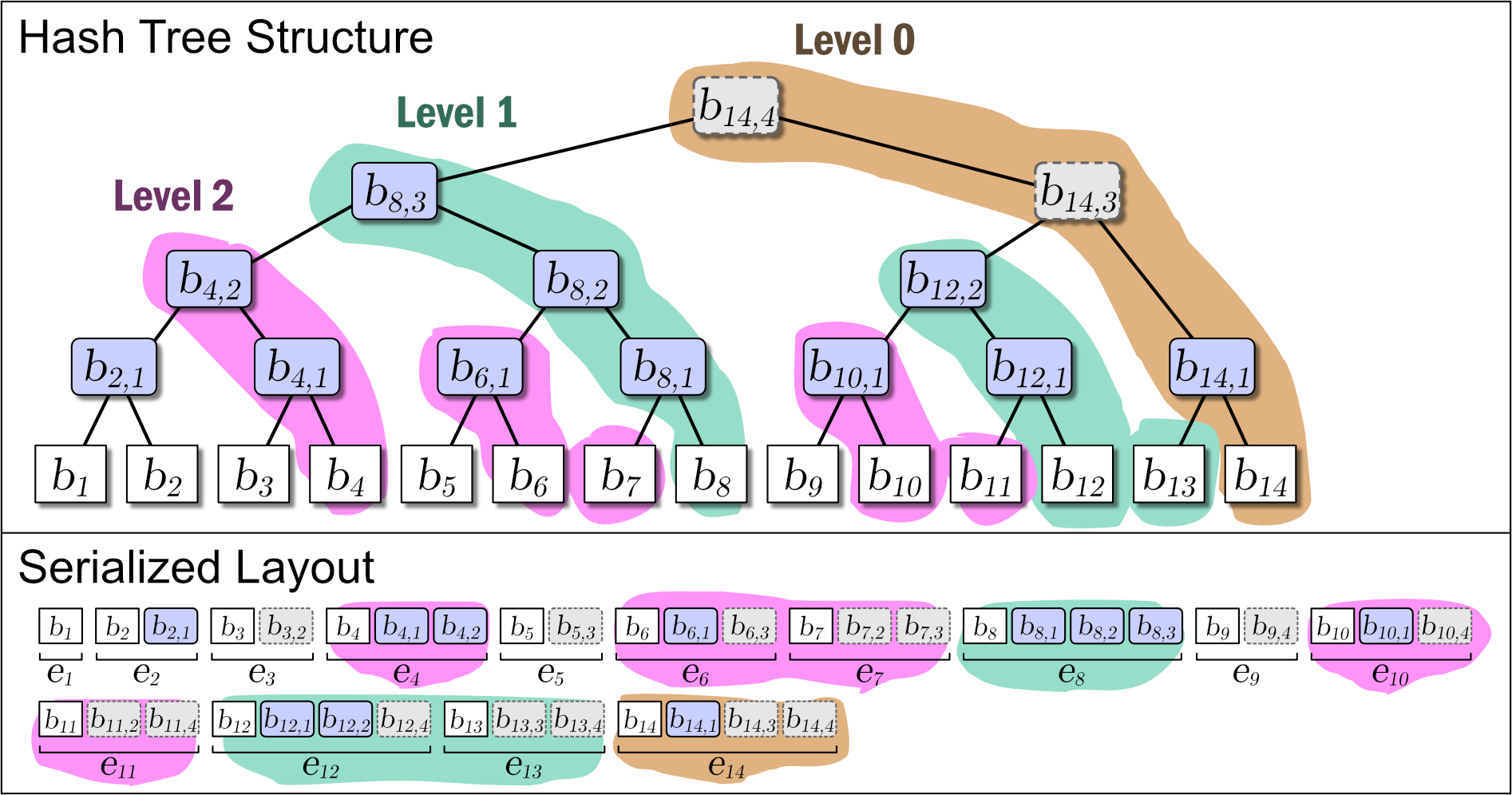
While Slate is not inherently a perfect binary tree, by growing and connecting the perfect binary tree substructures within it as leaf nodes are added, the majority of the nodes in the entire tree structure exhibit the properties of a perfect binary tree. Figure 1 shows the conceptual growth of the tree structure and its serialized format when data from 1 to 16 is added to Slate.
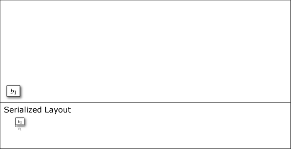
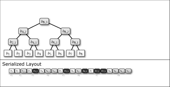
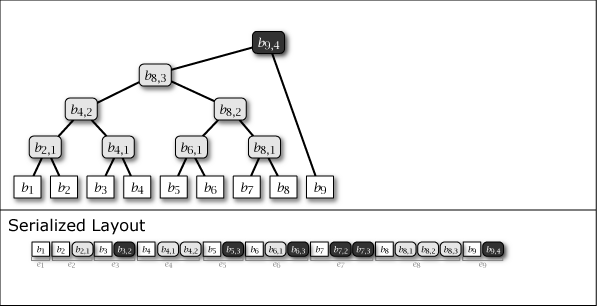
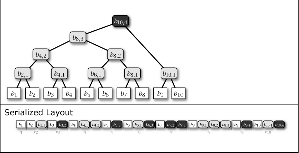
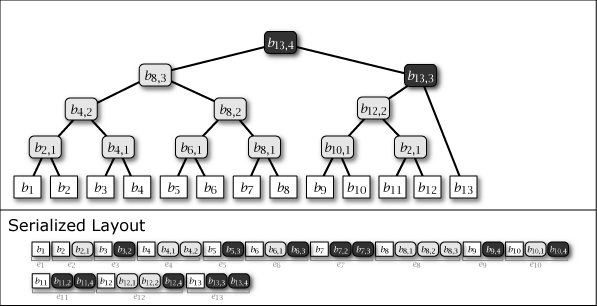
As Figure 1 shows, Slate's serialized representation is fast for file operations because it is an append-only operation. Also, since it retains the tree structure at any point in time as a complete history, it can respond with the correct hash tree even for data requests based on a past point in time.
Since Slate stores all versions of the tree structure, rollback and suffix replacement operations are also easy. When these operations are supported, Slate is no longer purely append-only, but it is designed on the premise that the majority of operations are appends. In this sense, the expression "append-optimized" is used.
Slate has the following features.
Persistent append-based growth list with verifiable hash tree. Slate is a data structure managed by a hash tree. It is optimized for applications with frequent appends, like time-series data, and is partially persistent at the data structure level. Like a normal hash tree, it can be used to detect the presence of data differences, corruption, or tampering, and to identify their location.
Append-optimized serialization with history revision support. It supports a serialization format for block devices like files and is particularly optimized for appends. It also supports rollback (truncate) to a certain version and suffix replacement to add new data from that point (note that while the data structure is persistent, the serialization format may have such changes).
Multi-versioned data structure. This tree structure is persistent, and a complete history of past structures is stored. Therefore, even if the tree grows due to data addition, the tree structure at any past point in time can be reproduced. If necessary, it is possible to roll back to a specific past version and resume from there.
Assign efficiency to more recent data. Slate's serialization format is designed to have locality such that the access efficiency of more recently added data is higher. The most recent data can be accessed with \(O(1)\) I/O operations (seek + read), and even the oldest data, the worst case, can be accessed with \(O(\log n)\) I/O operations. This is suitable for the realistic characteristic that more recently added data is accessed more frequently than older data.
Strength of safety over time. When considering the level of the authentication path (distance from the root node) as the strength of safety, the safety as a hash tree is asymmetric between elements that have existed for a long time and newly added elements. The strength of an element increases logarithmically each time another element is added, and when the whole becomes a perfect binary tree, all elements have the same reliability as a normal hash tree. This is a characteristic similar to a blockchain where the reliability (finality) of past blocks increases with the addition of new blocks.
The basic operations of Slate are append and get. An extension is range scan. With only these operations, the serialization format is also persistent and parallel reading can be easily implemented. Truncate and suffix replacement are available as options. Delete can be performed by logical deletion, leaving only the hash value, but the means to verify the authenticity of that hash value is lost.
2 Related Work
The Stratified Hash Tree is a new data structure that integrates concepts from several established research areas. It cites persistent data structures, hash-based integrity verification, and locality of stratified data as foundational areas, and distributed version control systems as an application area that clarifies practical synchronization requirements and solution methods.
This section clarifies the theoretical positioning of the Stratified Hash Tree in each of these research areas and demonstrates the uniqueness and contribution of this research through comparison with existing methods.
2.1 Persistent and Versioned Data Structures
The theory of persistent data structures enables efficient access to multiple versions of data. Persistent data structures were systematically studied by Driscoll et al. [5]. This paper distinguishes between ephemeral structures, which lose history upon modification, and persistent structures, which are maintained for subsequent access. Their research focused on general-purpose persistence methods for arbitrary data structures, introducing two basic techniques: the fat node method and the node copying method. In contrast, our Stratified Hash Tree focuses only on appends on a tree structure that provides features of partial persistence. Also, unlike the general node copying method, which requires careful management of version stamps and multiple pointers, the Stratified Hash Tree achieves persistence simply through a hierarchical structure where each entry \(e_i\) contains all nodes created during the update operation \(i\). This design choice eliminates the need for complex pointer management from our Slate. Furthermore, the append-only nature of Slate is well-suited for recent applications where immutability and efficient verification are important, such as distributed transaction logs and blockchains. Instead of holding explicit version pointers like Driscoll et al.'s method, the Stratified Hash Tree implicitly encodes version information through its layered structure, and temporal locality is naturally preserved as spatial locality.
2.2 Hash-Based Integrity and Temporal Structures
Ensuring data integrity using hash functions was first proposed by Merkle [6] as a protocol for public-key cryptosystems. This is called a Merkle tree, and it enables efficient integrity verification by placing hash values of data in the leaf nodes and recursively storing the hash values of child nodes in the intermediate nodes. This basic structure was later widely adopted in digital signature systems [7] and various distributed systems.
Research on incorporating temporal elements into hash-based structures dates back to the work of Haber and Stornetta [2] on digital document timestamping. They made it possible to prove the existence time of a document by linking the hash values of documents in chronological order. This method was improved by Bayer et al. [8] based on a hash tree, enabling efficient timestamping of multiple documents.
A more rigorous theoretical foundation was established by Buldas and Saarepera [8]. They proposed the concept of a hash calendar and developed a method to measure the passage of time by adding one hash value to an append-only database every second. This structure is positioned as a special Merkle tree and has the property that at any point in time, the tree contains a leaf node corresponding to each second since January 1, 1970. Buldas et al. [9] put this method into practice as a Universally Composable timestamping scheme, building a system that minimized dependence on a trusted third party.
These existing methods all provide an important foundation of combining hash-based integrity assurance and temporal elements. However, from the perspective of efficient synchronization of distributed transaction logs, they have the following limitations.
While Merkle trees provide excellent integrity verification functions, they do not perform structural optimization considering temporal locality. Since all leaf nodes are treated equally, high-frequency access patterns to recently added data cannot be exploited. Also, when new data is added, the entire tree may need to be rebalanced, which poses a challenge to efficiency in an append-only environment. In particular, when the number of data items is not a power of \(2^i\), it is necessary to create blank nodes or leaf nodes with special padding values, which increases implementation complexity and reduces storage efficiency.
The hash calendar is excellent as a temporally ordered append-only tree structure and is, in fact, the data structure most similar to the Stratified Hash Tree proposed in this document. Both adopt a common tree growth pattern of sequentially adding leaf nodes from left to right and gradually building upper-level nodes through the connection of perfect binary trees by ephemeral nodes. However, while the hash calendar focuses on timestamping and temporal integrity verification, the Stratified Hash Tree in this document addresses a different problem: efficient difference detection in distributed systems. Specifically, the design of placing one fixed hash value for each second in the hash calendar is not suitable for transaction logs with irregular update frequencies. Furthermore, efficient difference detection between multiple data streams with different update frequencies, the serialization representation of the tree, data locality, and temporal optimization are not discussed.
In contrast, the Stratified Hash Tree proposed in this document inherits the advantages of these existing methods while introducing optimizations favorable for distributed transaction log synchronization. Specifically, it achieves high-speed access to recent data through a hierarchical structure that utilizes temporal locality and enables efficient difference detection while maintaining append-only characteristics. It also provides adaptive hierarchy management functions to handle irregular update patterns, achieving practical distributed synchronization performance that was difficult to realize with existing Merkle trees or hash calendars.
2.3 Stratified Data Structures
Optimization by stratification is a design method that aims to improve overall performance by providing multiple layers according to the characteristics and usage patterns of the data. This concept is based on the principle of the memory hierarchy and improves system efficiency by leveraging differences in access frequency and temporal locality.
The Stratified B-Tree, proposed by Twigg et al. in 2011, is a data structure for versioned dictionaries [Twigg et al., 2011]. It was developed to solve the inefficiency of Copy-on-Write B-Trees. The Stratified B-Tree enables sequential I/O during updates and range queries by placing Key-Value pairs in layers of arrays, while maintaining density to avoid unnecessary duplication. It is similar to the Stratified Hash Table in this document in the sense of a layered data structure, but the two differ fundamentally in their axis of stratification. Whereas the Stratified B-Tree uses layers as independently managed version spaces, our Stratified Hash Tree separates the temporal order and uses layers as units with temporal locality. However, there is a conceptual similarity in that layers can also be used as versions in the Stratified Hash Tree.
The LSM-Tree (Log-Structured Merge Tree) [1] is a layered data structure optimized for write-intensive workloads. The LSM-Tree efficiently handles write operations by combining a structure in memory (memtable) and multiple levels of structures on disk (SSTable). New data is first added to the in-memory structure, and when it reaches a certain size, it is flushed to a lower level on disk. A periodic compaction process merges data between multiple levels, removing duplicates and optimizing space efficiency. This hierarchical approach is widely adopted in modern NoSQL databases such as Cassandra, HBase, and RocksDB. The concept of layers in the LSM-Tree is common with the Stratified Hash Tree in this document in terms of write optimization and layer management, but while the LSM-Tree mainly focuses on storage efficiency and write performance, the Stratified Hash Tree is optimized for difference detection and synchronization efficiency.
The concept of hierarchical storage management is a method in storage systems where data is placed in storage tiers with different performance characteristics according to the access frequency and importance of the data. By combining multiple tiers, from fast but expensive and small-capacity SSDs to slow but cheap and large-capacity HDDs and tape storage, the balance between cost-effectiveness and performance is optimized. This principle of stratification improves overall efficiency by utilizing temporal and spatial locality, placing frequently accessed data in high-speed tiers and archival data in low-speed tiers.
These existing layered data structures all share a common design philosophy of efficiency through layering, but each is specialized for a different problem domain. The Stratified B-Tree is mainly for versioned dictionaries, the LSM-Tree for write-intensive storage, and hierarchical storage for cost-effective large-capacity storage. The Stratified Hash Tree in this document converts these layering concepts so that temporal locality becomes spatial locality, providing an optimization that improves the access efficiency of recent data in an append-only environment.
2.4 Transaction Logs and Distributed Versioned Synchronization
Efficient data synchronization and consistency assurance in a distributed environment are fundamental challenges in modern distributed systems. In this field, consensus algorithms, distributed version control, delta synchronization techniques, and distributed ledger technologies have developed in interrelation with each other.
Raft was designed as an alternative to the Paxos algorithm to achieve consensus in distributed systems [Ongaro & Ousterhout, 2014]. It is designed to be easier to understand than Paxos by eliminating complexity and has been formally proven to be safe. Raft implements consensus through a leader approach, where a single leader elected in the cluster is responsible for managing log replication with other servers. In modern distributed SQL databases like TiDB and YugabyteDB, each data unit is replicated to other nodes using Raft. The process of leader election, log replication, and commit processing ensures data consistency even in the event of node failures or network partitions.
When a leader change occurs in Raft, to know how far a follower's log is synchronized with the new leader's log, the logs are compared one by one from the end. This method is simple, but in the worst case, it may require a linear operation of the entire log, which is \(O(n)\), and can be a performance problem for large logs.
Git is a practical implementation example of a distributed version control system. In Git, the history of a repository is represented as a DAG (Directed Acyclic Graph) structure, where each commit has a pointer to its parent commit(s). The detection of a branch's divergence point is realized by the git merge-base algorithm, which identifies the common ancestor (lowest common ancestor: LCA) of two branches. During a rebase operation, Git finds the common ancestor of two branches in the DAG and applies the changes from each commit of one branch on top of the other branch. However, this method detects the divergence point by a linear search from the back of the branch.
The rsync algorithm, a representative example of Delta Synchronization, is a fundamental technology for efficient differential transfer [Tridgell, 1999]. rsync minimizes network bandwidth consumption by synchronizing only the changed parts within a file. This is done by dividing the file into chunks on both the client and remote server and exchanging their checksums to transfer only the differences. This approach is efficient but is limited to file-level processing and is not suitable for hierarchical difference detection of structured data.
The lightweight clients of blockchain are an important example of the lightweighting brought about by hash-based verification. In Bitcoin's Simplified Payment Verification (SPV), the client downloads only the block headers, not all blocks, and relies on Merkle proofs to verify transactions. When an SPV client needs a transaction, it requests a Merkle proof from a full node to prove that the specific transaction obtained is included in the block. By hashing these values and comparing them with the Merkle root in the block header, it can be confirmed that the transaction is part of the block. However, SPV is mainly specialized for proof of inclusion and does not provide efficient differential synchronization functionality between multiple nodes.
These existing methods each provide solutions for specific synchronization or verification requirements, but they have limitations while sharing a common perspective of efficient difference detection of distributed transaction logs. The linear search of Raft and Git is intuitive but can be inefficient for large histories. The file-level synchronization of rsync is specialized for block devices and is not suitable for structured data. The verification of blockchain lightweight clients is sporadic and not optimized for continuous difference tracking.
The Stratified Hash Tree proposed in this document has the potential to solve these constraints. With its hierarchical structure that utilizes temporal locality, it can be expected to achieve \(O(\log n)\) efficiency in the worst case for Raft's log synchronization and Git's divergence point detection. Also, in rsync, hierarchical difference detection realizes a precision beyond conventional block-level synchronization, and in a blockchain environment, a reduction in computational complexity for continuous block verification is expected. These improvements are expected to lead to performance improvements compared to existing methods.
3 Preliminaries and Definitions
4 The Slate Data Structure
A Stratified Hash Tree is a binary tree in which perfect binary trees occupy most of its area. In this document, the entire tree structure of a Slate containing \(n\) user data (leaf nodes) is denoted by \(T_n\), the fact that a node \(b\) is included in a tree structure \(T\) is conveniently denoted by \(b \in T\), and that \(T_1\) is a subtree of \(T_2\) is denoted by \(T_1 \subseteq T_2\). Also, when focusing on the growth process of \(T_n\), it is expressed as the \(n\)-th generation.
Slate grows by integrating one or more perfect binary trees contained as substructures. Also, since most of the tree structure is a perfect binary tree, it has characteristics close to those of a perfect binary tree. Therefore, to utilize the features of Slate, a method to determine the perfect binary trees from the entire tree structure is important. Here, we describe the mathematical background necessary for the realistic operation of the Slate structure.
4.1 Nodes
User data is stored in the leaf nodes of Slate. Here, let \(i \in \{1,2,\ldots\}\) be the index of the user data, and the \(i\)-th leaf node added to Slate is represented as \(b_i\) (or more generally, it can also be written as \(b_{i,0}\)).
The intermediate nodes that occur when adding the \(i\)-th leaf node \(b_i\) to the existing tree structure \(T_{i-1}\) are denoted as \(b_{i,j}\). Here, \(j \in \{1,2,\ldots\}\) represents the distance to the farthest leaf node (height or depth) when considering the subtree rooted at \(b_{i,j}\). Therefore, the node with the largest \(j\) in the entire tree structure is its root node. Also, in any subtree rooted at \(b_{i,j}\), the case where \(j\) is the largest is when that subtree is a perfect binary tree, so the maximum value of \(j\) that the root node can take is \(\lceil \log_2 i \rceil\). Note that a single leaf node with \(j=0\) is also considered a subtree. \[ \begin{equation} i \in \{1,2,\ldots\}: 0 \le j \le \lceil \log_2 i \rceil \label{ij} \end{equation} \]
Equation (\(\ref{ij}\)) means that in a realistic implementation, even if the domain of \(i\) is a 64-bit integer, the maximum possible value of \(j\) is at most 64.
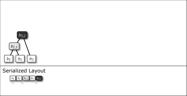
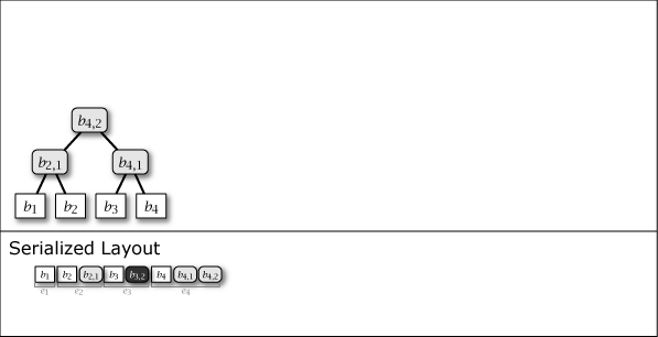
As shown in purple and light gray in Figure 1, there are two types of intermediate nodes. One is the case where the subtree rooted at that intermediate node is a perfect binary tree, which is persistent and will be present in all tree structures from the \(i\)-th generation onwards. The other is the case where it is not a perfect binary tree, which is an ephemeral intermediate node that appears only in the \(i\)-th generation, installed to connect the subtrees of other perfect binary trees. Ephemeral intermediate nodes are omitted in Figure 1 to simplify the explanation, but they always exist in the serialized format, and their tree structure can be restored at any time.
To indicate that an intermediate node \(b_{i,j}\) connects \(b_{i_\ell,j_\ell}\) to its left branch and \(b_{i_r,j_r}\) to its right branch, we write \(\underset{(i_\ell,j_\ell)(i_r,j_r)}{b_{i,j}}\).
4.2 Evaluating Perfect Binary Trees
Let \(T_{i,j} \subseteq T_n\) be the subtree (including leaf nodes) rooted at a node \(b_{i,j}\) contained in the tree structure \(T_n\). If there exists an integer \(\alpha\) such that equation (\(\ref{pbt}\)) holds for \(i,j\), then this subtree structure \(T_{i,j}\) is a perfect binary tree. \[ \begin{equation} i = \alpha \times 2^j \label{pbt} \end{equation} \] Here, \(\alpha \ge 1\) means which subtree it is from the beginning among the perfect binary trees \(T_{*,j} \subseteq T_n\) with the same height \(j\). When we intend for \(T_{i,j}\) to be a perfect binary tree, we add a \('\) (prime) and write \(T'_{i,j}\), and similarly, when we intend the root node of a subtree that becomes a perfect binary tree, we write \(b'_{i,j}\). Also, in the equations, a subtree that becomes a perfect binary tree is denoted as \({\rm PBST}\) (perfect binary subtree).
In implementation, it is possible to determine whether \(T_{i,j}\) is a perfect binary tree using only bitwise operations on the indices with equation (\(\ref{pbst}\)) derived from equation (\(\ref{pbt}\)). \[ \begin{equation} \begin{cases} i \equiv 0 \pmod{2^j} & \quad \text{If $T_{i,j}$ is a PBST} \\ i \not\equiv 0 \pmod{2^j} & \quad \text{Otherwise} \end{cases} \label{pbst} \end{equation} \] Here, \(x \bmod 2^y\) for integers \(x\), \(y\) can be expressed using the bitwise operator as x & ((1 << y) - 1). Also, it is clear that if \(j=0\), equation (\(\ref{pbst}\)) is always true, so any leaf node \(b_i = b_{i,0}\) is equivalent to a perfect binary tree.
4.3 Enumerating Independent Perfect Binary Subtrees
Consider a method to enumerate the independent (not substructures of each other) perfect binary trees contained in a tree structure \(T_n\) containing \(n\) leaf nodes (in the \(n\)-th generation).
Such perfect binary trees are arranged in order from the left, such that they are the largest perfect binary tree that can be constructed using the leaf nodes located to the right of that position (the remaining leaf nodes become the "material" for the next perfect binary tree). And since the largest perfect binary tree that can be constructed using \(x\) leaf nodes has a height of \(j=\max\{j\in\mathbb{Z}\mid 2^j\le x\}\) and \(2^j\) leaf nodes, it can be found by the following algorithm. Here, let \(\mathcal{B}'_n\) be the set of root nodes of the independent perfect binary trees contained in \(T_n\).
| 1. | \( {\bf function} \ {\rm pbst\_roots}(n:{\it Int}) \to {\it Sequence}[{\it Node}] \) | |
| 2. | \( \hspace{12pt}x := n \) | |
| 3. | \( \hspace{12pt}\mathcal{B}'_n := \emptyset \) | |
| 4. | \( \hspace{12pt}{\bf while} \ x \ne 0 \) | |
| 5. | \( \hspace{24pt}j = \max \{j \in \mathbb{Z} \mid 2^j \le x\} \) | |
| 6. | \( \hspace{24pt}\mathcal{B}'_n := \mathcal{B}'_n \mid\mid b'_{n-x+2^j,j} \) | // \(b'_{n-x+2^j,j}\) は完全二分木となる部分構造のルート |
| 7. | \( \hspace{24pt}x := x - 2^j \) | |
| 8. | \( \hspace{12pt}{\bf return} \ \mathcal{B}'_n \) | |
Here, let \(\mid\mid\) be the operator that concatenates ordered sets (list structures). Let the set of \(m\) perfect binary tree root nodes obtained from Algorithm 1 be \(\mathcal{B}'_n=(b'_{i_1,j_1},\ldots,b'_{i_m,j_m})\). Since these are ordered from the left in terms of placement, we have \(i_1 \lt \ldots \lt i_m\). Also, since the perfect binary tree located on the left is taller, we have \(j_1 \gt \ldots \gt j_m\).
4.4 Enumerating Ephemeral Nodes
The ephemeral intermediate nodes in Slate are formed by connecting the root nodes of the independent perfect binary trees, which are subtrees of \(T_n\), from the right. Therefore, by enumerating the independent perfect binary trees, the ephemeral intermediate nodes can also be enumerated.
For the set of \(m\) perfect binary tree root nodes \(\mathcal{B}'_n\) obtained from Algorithm 1, the ephemeral intermediate nodes that connect them are \(\mathcal{B}_n=(b_{n,j_1+1},\ldots,b_{n,j_{m-1}+1})\). Here, any ephemeral intermediate node located at the \(k\)-th position from the left is expressed as in equation (\(\ref{ephemeral_node}\)). \[ \begin{equation} \left\{ \begin{array}{ll} \underset{(i_k,j_k)(n,j_{k+1}+1)}{b_{n,j_k+1}} \ \ & (k \lt m - 1) \\ \underset{(i_k,j_k)(i_m,j_m)}{b_{n,j_k+1}} \ \ & (k = m - 1) \end{array} \right. \label{ephemeral_node} \end{equation} \] The ephemeral intermediate node represented by equation (\(\ref{ephemeral_node}\)) connects the perfect binary tree \(b'_{i_k,j_k}\) to its left branch, and the ephemeral node \(b_{n,j_{k+1}+1}\) or the rightmost perfect binary tree \(b'_{i_m,j_m}\) to its right branch. Since it is an ephemeral intermediate node in the \(n\)-th generation, \(i=n\), and since the binary tree connected to the left branch is always taller than the binary tree connected to the right branch, \(j=j_k+1\). Algorithm 2 is an algorithm that generates ephemeral intermediate nodes.
| 1. | \( {\bf function} \ {\rm ephemeral\_nodes}(n:{\it Int}) \to {\it Sequence}[{\it Node}] \) | |
| 2. | \( \hspace{12pt}\mathcal{B}'_n := {\rm pbst\_roots}(n) \) | // Algorithm 1 |
| 3. | \( \hspace{12pt}\mathcal{B}_n := \emptyset \) | |
| 4. | \( \hspace{12pt}{\bf for} \ x := {\rm size}(\mathcal{B}'_n)-1 \ {\bf to} \ 1 \) | |
| 5. | \( \hspace{24pt}i = n, \) | |
| 6. | \( \hspace{24pt}j = \mathcal{B}'_n[x].j+1 \) | |
| 7. | \( \hspace{24pt}left = \mathcal{B}'_n[x-1] \) | |
| 8. | \( \hspace{24pt}right = \mathcal{B}_n[0] \ {\bf if} \ x \ne {\rm size}(\mathcal{B}'_n)-1 \ {\bf else} \ \mathcal{B}'_n[x] \) | |
| 9. | \( \hspace{24pt}\mathcal{B}_n := b \{i, j, left, right\} \ \mid\mid \ \mathcal{B}_n \) | |
| 10. | \( \hspace{12pt}{\bf return} \ \mathcal{B}_n \) | |
From this tree construction procedure, when considering the nodes \(b_{i_l,j_l}\) and \(b_{i_r,j_r}\) connected to the left and right branches of any node \(b_{i,j} \in T_n\), the nodes of Slate have the following trivial properties.
Property 1: The subtree rooted at the node \(b'_{i_l,j_l}\) connected to the left branch of any node \(b_{i,j} \in T_n\) is a perfect binary tree. Also, the subtree rooted at the node \(b_{i_r,j_r}\) connected to the right branch may be a perfect binary tree.
Property 2: The height of the node \(b_{i_l,j_l}\) connected to the left branch of any node \(b_{i,j} \in T_n\) is \(j_l = j - 1\).
Property 3: The index of the node \(b_{i_r,j_r}\) connected to the right branch of any node \(b_{i,j} \in T_n\) is \(i_r = i\). Also, considering this property recursively, a series of nodes that follow the right branch of any node down to a leaf node have the same value of \(i\).
Also, a script to find the sets \(\mathcal{B}'_n\) and \(\mathcal{B}_n\) from \(n\) based on Algorithm 1 and Algorithm 2 is shown below.
Since operations on the \(n\)-th generation \(T_n\) frequently refer to the nodes contained in \(\mathcal{B}'_n\) and \(\mathcal{B}_n\), it would be good to cache these in memory.
4.5 Indexing
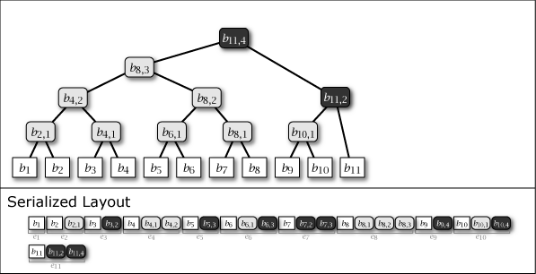
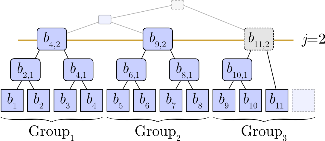
Slate has the property of a hierarchical structure that divides data into groups of \(2^j\). In generation \(n\), a completely filled group means that the corresponding subtree is a perfect binary tree. For example, at height \(j=2\), it becomes a group of capacity 4, and for \(n=11\), two groups are completely filled and one group is not. \[ \begin{array}{lll} {\rm Group}_1 &\ = &\ (1, 2, 3, 4) &\quad \text{completely filled (PBST)} \\ {\rm Group}_2 &\ = &\ (5, 6, 7, 8) &\quad \text{completely filled (PBST)} \\ {\rm Group}_3 &\ = &\ (9, 10, 11, \_) &\quad \text{not completely filled (not PBST)} \end{array} \] Representing this as a tree structure gives Figure 2.
4.5.1 Number of Leaf Nodes in an Arbitrary Subtree
We find the number of leaf nodes \(r_{i,j}\) contained in the subtree \(T_{i,j}\) rooted at an arbitrary node \(b_{i,j}\). First, if the subtree \(T'_{i,j}\) is a perfect binary tree (\(i \equiv 0\pmod{2^j}\)), the \(\frac{i}{2^j}\)-th group corresponding to \(T_{i,j}\) is full, and since each group has a capacity of \(2^j\), we have \(r'_{i,j}=2^j\).
Next, if the subtree \(T_{i,j}\) is not a perfect binary tree (\(i \not\equiv 0 \pmod{2^j}\)), that is, it is rooted at an ephemeral node \(b_{i,j}\), the tree corresponds to the \(\lfloor \frac{i}{2^j}\rfloor\)-th group, and before it, there are \(\lfloor\frac{i}{2^j}\rfloor\) full groups. Therefore, \(r_{i,j}=i-\lfloor\frac{i}{2^j}\rfloor\times 2^j\). \[ \begin{equation} \begin{cases} r'_{i,j} & = & 2^j & \quad i \equiv 0 \pmod{2^j} \\ r_{i,j} & = & i - \left\lfloor\frac{i}{2^j}\right\rfloor \times 2^j & \quad i \not\equiv 0 \pmod{2^j} \end{cases} \label{r_cases} \end{equation} \]
In the case of a perfect binary tree, \(i \equiv 0 \pmod{2^j}\) means that there exists an integer \(q \ge 1\) such that \(i = q \times 2^j\). Also, since \(q-1\) represents the number of the previous group, we have \(q-1=\lfloor \frac{i-1}{2^j} \rfloor\). Therefore, \(r'_{i,j}\) can be transformed as in Equation (\(\ref{r_pbst}\)). \[ \begin{eqnarray} r'_{i,j} & = & 2^j = q \times 2^j - (q - 1) \times 2^j \nonumber \\ & = & i - \left\lfloor\frac{i-1}{2^j}\right\rfloor \times 2^j \label{r_pbst} \end{eqnarray} \] Also, for \(i \not\equiv 0 \pmod{2^j}\), we have \(\lfloor\frac{i}{2^j}\rfloor = \lfloor\frac{i-1}{2^j}\rfloor\), so \(r_{i,j}\) can also be transformed as in Equation (\(\ref{r_ephemeral}\)). \[ \begin{eqnarray} r_{i,j} & = & i - \left\lfloor \frac{i}{2^j} \right\rfloor \times 2^j \nonumber \\ & = & i - \left\lfloor \frac{i-1}{2^j} \right\rfloor \times 2^j \label{r_ephemeral} \end{eqnarray} \] Thus, the case distinction in Equation (\(\ref{r_cases}\)) can be integrated into Equations (\(\ref{r_pbst}\), \(\ref{r_ephemeral}\)). Here, \(\lfloor\frac{i-1}{2^j}\rfloor\) represents the number of groups that exist before \(T_{i,j}\).
In general, for any integers \(a\), \(b\) (\(b\gt 0\)), since \(a = \lfloor\frac{a}{b}\rfloor \times b + (a \bmod b)\), applying \(a=(i-1)\) yields Equation (\(\ref{r}\)). \[ \begin{eqnarray} r_{i,j} & = & i - \left\lfloor \frac{i-1}{2^j} \right\rfloor \times 2^j \nonumber \\ & = & ((i - 1) \bmod 2^j) + 1 \label{r} \end{eqnarray} \] With this Equation (\(\ref{r}\)), the number of leaf nodes \(r_{i,j}\) contained in any node \(b_{i,j}\) can be calculated uniformly, regardless of whether it is a perfect binary tree or an ephemeral node.
4.5.2 Subtree Coverage Range
Consider the index range \([i_{\rm min}, i_{\rm max}]\) of the leaf nodes contained in an arbitrary subtree \(T_{i,j} \subseteq T_n\). From Property 3, it is clear that the maximum index is \(i_{\rm max} = i\), so we focus on the minimum index \(i_{\rm min}\).
Before the subtree \(T_{i,j}\) of height \(j\), regardless of whether \(T_{i,j}\) is a perfect binary tree, there are \(\lfloor\frac{i-1}{2^j}\rfloor\) subtrees (perfect binary trees) \(T'_{i',j}\), \(i' \lt i\) of the same height \(j\). Since a perfect binary tree of height \(j\) contains \(2^j\) leaf nodes, the minimum index \(i_{\rm min}\) of \(T_{i,j}\) can be considered as the total number of leaf nodes existing before \(T_{i,j}\) + 1. \[ \begin{equation} \left\{ \begin{array}{lcl} i_{\rm min} & = & \left\lfloor \frac{i-1}{2^j} \right\rfloor \times 2^j + 1 = i - ((i-1)\bmod 2^j) \\ i_{\rm max} & = & i \end{array} \right. \label{subtree_range} \end{equation} \] From Equation (\(\ref{subtree_range}\)), the number of leaf nodes contained in \(T_{i,j}\) is \(i_{\rm max}-i_{\rm min}+1=r\), which matches Equation (\(\ref{r}\)). Also, the "maximum leaf node of the adjacent subtree to the left" and the "minimum leaf node of the adjacent subtree to the right" of \(T_{i,j}\) can also be calculated. This idea is used in the explanation of connecting intermediate nodes.
Here, \(\lfloor\frac{x}{2^y}\rfloor\) for integers \(x\), \(y\) can be expressed using the bitwise operator as x >> y, and similarly \(x \times 2^y\) can be expressed as x << y.
4.5.3 Indices of Left and Right Nodes
Consider the nodes \(b_{i_l,j_l}\) and \(b_{i_r,j_r}\) connected to the left and right branches of an arbitrary node \(b_{i,j} \in T_n\). From Property 2 and Property 3, it is clear that \(j_l = j-1\) and \(i_r=i\), so we find the remaining \(i_l\) and \(j_r\).
First, we find \(i_l\).
\(T_{i_l,j-1}\) shares the leftmost leaf node with \(T_{i,j}\). That is, the number of leaf nodes before \(T_{i_l,j-1}\) is the same as the number of leaf nodes before \(T_{i,j}\), and that number is \(i_{\rm min}-1=\lfloor\frac{i-1}{2^j}\times 2^j\) from Equation (\(\ref{subtree_range}\)).
From Property 1, \(T_{i_l,j-1}\) is a perfect binary tree of height \(j-1\). Therefore, \(T_{i_l,j-1}\) contains \(2^{j-1}\) leaf nodes.
Therefore, the rightmost leaf node of \(T_{i_l,j-1}\) has \(i_l = \lfloor\frac{i-1}{2^j}\rfloor\times 2^j + 2^{j-1}\).
Next, since the number of leaf nodes contained in \(T_{i,j_r}\) is \(i-i_l\), the height of \(T_{i,j_r}\) can be calculated as \(j_r=\lceil\log_2(i-i_l)\rceil\). In summary, the left and right nodes \(b_{i_l,j_l}\), \(b_{i_r,j_r}\) at an arbitrary node \(b_{i,j} \in T_n\) can be expressed as in Equation (\(\ref{lr_index}\)). \[ \begin{equation} \begin{cases} (i_l, j_l) & = & \left(\left\lfloor \frac{i-1}{2^n} \right\rfloor \times 2^j + 2^{j-1}, j-1\right) \\ & = & (i-((i-1)\bmod 2^j)+2^{j-1}-1, j-1) \\ (i_r, j_r) & = & (i, \left\lceil \log_2(i-i_l) \right\rceil) \end{cases} \label{lr_index} \end{equation} \]
4.6 Height of Intermediate Nodes
There are two cases where the subtree structure \(T_{i,j}\) in Slate does not become a perfect binary tree. One is when \(b_{i,j}\) connects two perfect binary trees of different heights to its left and right branches, and the other is when the right branch of \(b_{i,j}\) (the side containing the larger \(i\)) is not a perfect binary tree. Note that the subtree connected to the left branch of any intermediate node is a perfect binary tree. That is, the two subtrees connected by any \(b_{i,j}\) are either of equal level (if \(T_{i,j}\) is a perfect binary tree), or the subtree connected to the left branch is larger (if \(T_{i,j}\) is not a perfect binary tree). Therefore, if the subtree connected to the left branch of a new intermediate node \(b_{i,j}\) is \(T'_{k,\ell}\), then \(j=\ell+1\).
4.7 Serialized Representation
When adding the \(i\)-th value \(b_i\) to Slate, one leaf node \(b_i\) and zero or more intermediate nodes \(b_{i,j}\) are generated. These node informations are collected, and the element added \(i\)-th to the serialized representation \(S\) of Slate is represented as entry \(e_i\). These are arranged as in the Serialized Layout of Figure 1. Here, the node placed at the far right of \(S\) is always the root node of Slate.
Entry \(e_i\) contains all nodes \(b_{i,*}\) that have the same generation. In addition, since the node connected to the right branch of an intermediate node is of the same generation, the case of searching the node to the right branch side can be completed with one entry read. In other words, Slate has the characteristic that access to more recent user data is more efficient.
4.8 Search Efficiency
As mentioned above, in the serialized format of Slate, all nodes added in a certain generation are contained in the same entry. In other words, the right-side node \(b_{i,y}\) of any intermediate node \(b_{i,x}\) is contained in the same entry as \(b_{i,x}\), which means that a search to the right-side branch can be done with a single seek + read on the storage. Therefore, the worst case is a case where all movements from the root node are to the left-side branch, that is, when searching for the oldest data. In such a worst case, the number of seek + read operations to read the oldest entry is \(O(log_2 N)\).
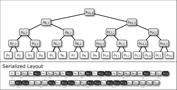
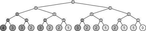
To give a specific example, if only the latest entry is cached in memory, the number of seek + read operations to reach each node contained in the tree structure of \(T_{16}\) is as shown in Figure 3.
5 Operations and Algorithms
Let \(S\) be the list structure that is the serialized representation of Slate, and let \(S[x]\) be the node stored at the \(x\)-th position of \(S\). In particular, the notation \(S[{\rm last}]\) represents the last node of \(S\).
5.1 Append Operation
The operation to add a new leaf node \(b_i\) to \(S\) constructs the entry \(e_i\) using Algorithm 1 and Algorithm 2 and concatenates it to \(S\).
- Construct \(e_i\) using the following set of nodes. Here, all nodes are assumed to be sorted in descending order of \(j\).
- Leaf node \(b_i\)
- Intermediate nodes that are \(b'_{i,*}\) contained in the ordered set \(\mathcal{B}'_i\) obtained by Algorithm 1
- All intermediate nodes of the ordered set \(\mathcal{B}_i\) obtained by Algorithm 2
- Concatenate \(e_i\) to \(S\).
The \(e_i\) created by this procedure places the leaf node \(b_i\) at the beginning of the node and the root node of the tree structure at the end of the node.
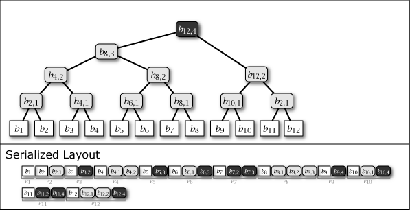
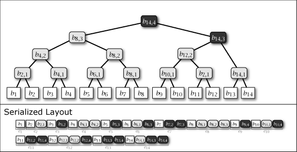
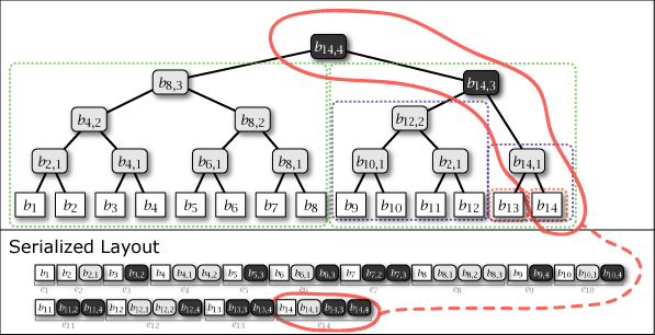
Figure 4 is the tree structure constructed as a result of performing the above operation to add \(b_{14}\) to \(T_{13}\). It can be seen that the intermediate node connects "the largest subtree containing the newly added \(b_i\)" and "the largest perfect binary tree located to the left of that subtree" and the entire tree structure is connected.
5.1.1 The \({\rm append}(e:{\it Node})\) Function
Algorithm 3 represents the operation of adding a new leaf node \(b_n\) to the serialized representation of an existing tree structure.
| 1. | \( {\bf function} \ {\rm append}(b_n:Node) \) | |
| 2. | \( \hspace{12pt}\mathcal{B}'_n = {\rm pbst\_roots}(n) \) | // Algorithm 1 |
| 3. | \( \hspace{12pt}\mathcal{B}_n = {\rm ephemeral\_nodes}(n) \) | // Algorithm 2 |
| 4. | \( \hspace{12pt}e_n = {\rm sort} \ (\{b_n\} \cup \{b_{i,*} \in \mathcal{B}'_n \mid i=n\} \cup \mathcal{B}_n) \ {\rm by} \ j \) | // \(j\) で降順ソートされた順序集合となるように |
| 5. | \( \hspace{12pt}S := S \mid\mid e_i \) | |
5.2 Retrieval Operations
Searching in Slate is the same as a normal binary tree search. In the special case where the entire tree structure is a perfect binary tree, all leaf nodes can be reached uniformly in \(O(\log_2 N)\), but otherwise, it has the characteristic that more recently added leaf nodes belong to a relatively low-level subtree, so that the latest data can be searched faster. However, in that case, an additional step of operation is required due to the existence of ephemeral intermediate nodes, so the generalized computational complexity for search is \(O(\lceil \log_2 N \rceil)\).
5.2.1 Single Element Search
5.2.1.1 The \({\rm contains}(b_{i,j}:{\it Node},k:{\it Int})\) Function
Equation (\(\ref{subtree_range}\)) can be used to determine which of the left and right branches of a binary tree search contains the target leaf node. By determining whether the leaf node \(b_k\) is contained in the subtree rooted at a node \(b_{i,j}\), it can be determined which of the left and right branches of the intermediate node contains the target leaf node.
| 1. | // Determine if the leaf node \(b_k\) is contained in the subtree structure rooted at \(b_{i,j}\) | |
| 2. | \( {\bf function} \ {\rm contains}(b_{i,j}:{\it Node}, k:{\it Int}) \to {\it Boolean} \) | |
| 3. | \( \hspace{12pt}i_{\rm min}, i_{\rm max} = {\rm range}(b_{i,j}) \) | |
| 4. | \( \hspace{12pt}{\bf return} \ i_{\rm min} \le k \ {\bf and} \ k \le i_{\rm max} \) | |
5.2.1.2 The \({\rm retrieve}(e:{\it Node},i:{\it Int})\) Function
Note that if append and search operations are performed in parallel in a multi-threaded/multi-process environment, \(S[{\rm last}]\) may not be the root node of Slate if it is executed during an append operation.
| 1. | \( b_i := {\rm retrieve}(S[{\rm last}], i) \) | |
| 2. | \( {\bf function} \ {\rm retrieve}(b_{i,j}:{\it Node}, k:{\it Int}) \to {\it Node} \) | |
| 3. | \( \hspace{12pt}{\bf if} \ j = 0 \ {\bf then} \) | |
| 4. | \( \hspace{24pt}{\bf return} \ {\bf if} \ i = k \ {\bf then} \ b_{i,j} \ {\bf else} \ {\it None} \) | |
| 5. | \( \hspace{12pt}{\bf else \ if} \ {\rm contains}(b_{i,j}.{\rm left}, k) \ {\bf then} \) | |
| 6. | \( \hspace{24pt}{\bf return} \ {\rm retrieve}(b_{i,j}.{\rm left}, k) \) | |
| 7. | \( \hspace{12pt}{\bf else} \) | |
| 8. | \( \hspace{24pt}{\bf return} \ {\rm retrieve}(b_{i,j}.{\rm right}, k) \) | |
5.2.2 Range Scan Operation
Since all elements are serialized on \(S\), range search is easy. To get the elements from \(t_0\) to \(t_1\), you just need to search for the position of \(b_{t_0}\) on \(S\) and then read \(S\) to the right until \(b_{t_1}\) is detected.
If the read position is \(i\), reading or skipping (seeking) 1 to \(\log_2 i\) intermediate nodes per element occurs, but the intermediate nodes themselves are not that large, and since it is a continuous area, it is considered that the I/O buffer will function effectively and there will be no major impact.
| 1. | \( {\bf function} \ {\rm range\_scan}(b_{i,j}:{\it Node}, i_{\rm min}:{\it Int}, i_{\rm max}:{\it Int}) \to \) | |
5.2.2.1 The \({\rm range}(b_{i,j}:{\it Node})\) Function
| 1. | \( {\bf function} \ {\rm range}(b_{i,j}:{\it Node}) \to ({\it Int}, {\it Int}) \) | |
| 2. | \( \hspace{12pt}i_{\rm max} = i \) | |
| 3. | \( \hspace{12pt}i_{\rm min} = (\lfloor 1/2^j \rfloor - (1 \ {\bf if} \ i \bmod 2^j = 0 \ {\bf else} \ 0)) \times 2^j + 1 \) | |
| 4. | \( \hspace{12pt}{\bf return} \ (i_{\rm min}, i_{\rm max}) \) | |
Note that since the range of \(j\) is \(0..\lceil \log_2 i \rceil\), if the domain of \(i\) is 64-bit, \(2^j\) can take a range of 65-bit values.
5.2.3 Retrieval with Hashes Operation
When searching for an element as a hash tree, not only the element itself but also the hash values of the intermediate nodes that branch from the path must be obtained. Let \(T_n\) be a tree structure rooted at \(b_{n,\ell}\), and consider the intermediate nodes required when retrieving all leaf nodes (user data) belonging to an arbitrary node \(b_{i,j} \in T_n\).
5.2.3.1 The \({\rm level}(b_{n,\ell}:{\it Node}, b_{i,j}:{\it Node})\) Function
The number of intermediate nodes required for the result of a search with hashes is equal to the level of \(b_{i,j}\) (the number of ancestors from \(b_{i,j}\) to the target root node \(b_{n,\ell}\)). If \(T_n\) is a perfect binary tree, it is clear that it is \(\ell - j\), but if not, it is necessary to heuristically find the distance to the perfect binary tree containing \(b_{i,j}\).
| 1. | \( {\bf function} \ {\rm level}(b_{n,\ell}:{\it Node}, b_{i,j}:{\it Node}) \to Int \) | |
| 2. | \( \hspace{12pt}{\bf if} \ {\bf not} \ {\rm contains}(b_{n,\ell}, i) \ {\bf then} \) | |
| 3. | \( \hspace{24pt}{\bf return} \ {\it None} \) | |
| 4. | \( \hspace{12pt}b := b_{n,\ell} \) | |
| 5. | \( \hspace{12pt}{\rm step} := 0 \) | |
| 6. | \( \hspace{12pt}{\bf while} \ b \ne b_{i,j} \ {\bf and} \ b.i \bmod 2^{b.j} \ne 0 \) | |
| 7. | \( \hspace{24pt}b := b.{\rm left} \ {\bf if} \ {\rm contains}(b.{\rm left}, i) \ {\bf else} \ b.{\rm right} \) | |
| 8. | \( \hspace{24pt}{\rm step} = {\rm step} + 1 \) | |
| 9. | \( \hspace{12pt}{\bf return} \ b.j - j + {\rm step} \) | |
This function can be used on the client side to verify that the server response contains the correct number of intermediate nodes (hash values).
5.2.3.2 The \({\rm retrieve\_with\_hashes}()\) Function
| 1. | \( {\bf function} \ {\rm retrieve\_with\_hashes}(b_{n,\ell}:{\it Node}, b_{i,j}:{\it Node}) \to ({\it Set}[{\it Node}], {\it Sequence}[{\it Node}]) \) | |
| 2. | \( \hspace{12pt}{\bf if} \ {\bf not} \ {\rm contains}(b_{n,\ell}, i) \ {\bf then} \) | |
| 3. | \( \hspace{24pt}{\bf return} \ {\it None} \) | |
| 4. | \( \hspace{12pt}b := b_{n,\ell} \) | |
| 5. | \( \hspace{12pt}{\rm branches} := \emptyset \) | |
| 6. | \( \hspace{12pt}{\bf while} \ b \ne b_{i,j} \) | |
| 7. | \( \hspace{24pt}{\bf if} \ {\rm contains}(b.{\rm left}, i) \ {\bf then} \) | |
| 8. | \( \hspace{36pt}b := b.{\rm left} \) | |
| 9. | \( \hspace{36pt}{\rm branches} := {\rm branches} \mid\mid b.{\rm right} \) | |
| 10. | \( \hspace{24pt}{\bf else} \) | |
| 11. | \( \hspace{36pt}b := b.{\rm right} \) | |
| 12. | \( \hspace{36pt}{\rm branches} := {\rm branches} \mid\mid b.{\rm left} \) | |
| 13. | \( \hspace{12pt}i_{\rm min}, i_{\rm max} = {\rm range}(b) \) | |
| 14. | \( \hspace{12pt}{\rm values} := {\rm range\_scan}(b, i_{\rm min}, i_{\rm max}) \) | |
| 15. | \( \hspace{12pt}{\bf return} \ ({\rm branches}, {\rm values}) \) | |
5.2.4 Calculating Branch Nodes
Find the distance from the root node of a \(T_n\) to an arbitrary \(b_{i,j} \in T_n\). Let the subtree containing \(b_{i,j}\) among the root nodes of the perfect binary tree substructure found by Algorithm 1 be \(b'_{i',\log_2 i'}\).
- Get the root node of the perfect binary tree containing the target node \(b_{i,j}\) and get the distance from the root node of \(T_n\).
- When the root node of the perfect binary tree is \(b'_{i',j'}\), calculate the distance \(j' - j\) from \(b'_{i',j'}\).
| 1. | \( {\bf function} \ {\rm nodes\_at\_branches}(n:{\it Int}, i:{\it Int}, j:{\it Int}) \to {\it Int} \) | |
| 2. | \( \hspace{12pt}\mathcal{B}'_n = {\rm Algorithm1}(n) \) | |
| 3. | \( \hspace{12pt}b := {\rm root \ of \ } T_n \) | |
| 4. | \( \hspace{12pt}{\bf for} \ b'_{i',j'} \ {\bf in} \ \mathcal{B}'_n \) | |
| 5. | \( \hspace{24pt}{\bf if} \ {\rm contains}(b'_{i',j'}, i, j) \) | |
5.3 Auxiliary Operations
5.3.1 Bootstrap Process
Since all operations frequently access the entry \(S[{\rm last}]\) containing the root node of the tree structure, it would be possible to operate efficiently by reading the contents of \(S[{\rm last}]\) at startup and holding it in memory. However, since reading sequentially from the beginning \(S[1]\) will take time when \(S\) becomes large, it should be possible to get \(S[{\rm last}]\) from the end of the file. This could be implemented as follows:
Put information at the end of the file that allows you to find the starting position of \(S[{\rm last}]\) with a fixed-length seek from the end of the file.
Put a checksum to confirm that the information from \(S[{\rm last}]\) to that information is correct.
To detect a situation where the node is correct but not all intermediate nodes have been written, confirm that the read \(S[{\rm last}]\) represents the entire tree structure.
If corruption of \(S[{\rm last}]\) is detected, the last correctly read element \(b_i\) from \(S[1]\) is taken as \(S[{\rm last}]\).
5.3.2 Rollback and Suffix Replacement Operations
The rollback operation is just to truncate the serialized storage to the position of a certain generation.
6 Complexity Analysis
7 Implementation Considerations
7.1 Cache Design
To efficiently execute append and search operations in Slate, it is necessary to strategically cache specific nodes of the tree structure. This section describes a cache design that considers the structural features of Slate.
7.1.1 Cache-Oblivious Properties
Although it cannot be asserted that Slate is a cache-oblivious algorithm in the strict sense, it is expected to have properties close to cache-oblivious from the following characteristics.
Locality in the serialization layout: All nodes of the same generation \(b_{i,*}\) are stored in the same entry \(e_i\), and a search in the right-branch direction is completed within a single memory block. This property benefits from locality regardless of the cache line size or page size.
Recursive perfect binary tree structure: The perfect binary trees \(T'_{i,j}\) contained in Slate can each be treated as an independent substructure. This can be said to be a hierarchical access pattern similar to the van Emde Boas layout. This allows for the natural utilization of hierarchical locality, regardless of the depth of the cache hierarchy.
Bias in access patterns: Slate has a structural feature where newer data is placed at a shallower position. This is consistent with the property of time-series data that "the more recent the data, the higher the access frequency." This bias functions effectively regardless of the cache size.
In the perfect binary trees contained in Slate, it has cache-obliviousness equivalent to a standard binary search tree, and even in the worst case (access to the oldest data), since it is suppressed to at most one cache miss at each level, the following conjecture is considered to hold.
Conjecture: Even without knowing the parameters of the memory hierarchy (cache size \(M\), block size \(B\)), the number of cache misses for a search operation in a Slate with \(n\) elements is \(O(\log_B n)\).
Due to such cache-oblivious properties, Slate is expected to exhibit efficient performance in various hardware environments without implementing explicit cache management. However, this property is a theoretical prediction, and a rigorous proof is a future task.
7.1.2 Phased Cache Strategy
The cache-oblivious properties in Slate are mainly features derived from data locality and are related to the reduction of disk I/O and the effective use of the CPU cache. On the other hand, in a realistic implementation, an explicit cache is recommended for the purpose of reducing computation.
Due to the excellent structural design of Slate, the latest entry \(e_n\) contains all the following information necessary to start the operation of the tree structure.
The root node of the current generation \(b_{n,\lceil \log n \rceil}\): This is the starting point for all operations.
Reference to the root node of the perfect binary tree: It is referenced (only the position, not the actual data) as the connection destination with the newly generated node in the append operation. Also, in a search operation, the position of the root of the perfect binary tree can be identified without I/O.
The set of ephemeral nodes \(\mathcal{B}_n\): Forms the tree structure of the current generation.
Due to this property, even if no cache is used at all, the operation of the tree structure can be started with a single read of the last entry \(e_n\) of the serialized representation \(S_n\).
In other words, just by caching the latest entry \(e_n\) in memory, the first read can be reduced in all major operations. The space complexity required to cache \(e_n\) is extremely small at \(O(\log n)\), and its effect appears as a uniform reduction of one I/O in every operation. Due to this high cost-effectiveness, caching the latest entry is strongly recommended.
In addition, for read-centric workloads, further performance improvement is possible by gradually expanding the cache range down the tree structure. Here, let the caching of the latest entry \(e_n\) mentioned above be level 0 (basic cache). A level \(k\) cache caches the entries containing nodes from the root of the perfect binary tree to a depth of \(k\). The space complexity is \(O(2^k \times (\log n)^2)\), but the upper limit of \(k\) is limited to the height of the tree \(\log_2 n\).
For example, level 1 caches each entry \(e_i\) containing each root node \(b'_{i,j} \in \mathcal{B}'_n\) of the perfect binary trees contained in \(T_n\). This makes it possible to start the search of the perfect binary tree without I/O, and one additional READ is reduced. The space complexity is \(O((\log n)^2)\). Furthermore, at level 2, each entry containing the left child node of the root node of each perfect binary tree is cached. The first branch in the perfect binary tree is now covered, and one more READ is reduced. In this way, a phased cache can be used adaptively for the search workload.
7.1.3 Implementation Recommendations
In many applications, a sufficient effect can be obtained with only the level 0 basic cache. In particular, for append-centric workloads or time-series data processing with frequent access to recent data, higher-level caches may not bring a valid effect.
On the other hand, for applications with a uniform access pattern over the entire data range, access to old data can also be accelerated by adopting a level 1 cache. Level 2 and above should be limited to special applications that require extremely low latency.
In this way, the cache design of Slate provides a basic strategy that can obtain an effect with a minimum amount of memory usage and a phased extension option according to the access pattern. Because the structure itself has locality, it has practical performance even without a cache, and a valid performance improvement can be realized with a simple cache strategy.
As an additional option, it is conceivable to heuristically cache the recently accessed entries (e.g., by LRU) or the set of nodes of a generation that is known to be frequently accessed, but since its effectiveness depends on the access pattern of the application, it is omitted here.
7.2 Concurrency Control
In a practical system, concurrent access from multiple processes or threads is assumed. In particular, for applications such as transaction logs and blockchains, concurrency is essential. The structural properties of Slate are particularly advantageous in a concurrent processing environment. Multiple processes can access the data in parallel for the part of the subtree that has been finalized and all written nodes and their associated tree structure have become persistent.
7.2.1 Safety of Parallel Reading
If up to generation \(n\) is finalized (no truncate or replace occurs), then neither the tree structure \(T_n\) nor the serialized representation \(S_n\) will change in value or structure. Therefore, read operations can be performed completely independently of append operations.
Stability of finalized entries: Once an entry is written, it is not changed.
The fact that the elements written to Slate and the associated tree structure are persistent is advantageous for concurrent processing. Although the addition of elements and intermediate nodes to the serialized representation \(S\) needs to be done by a single process, searches can be performed safely even while append operations or other search operations are in progress, by performing them based on the finalized tree structure at the time the search starts.
7.2.2 Avoiding Write Conflicts
The addition of a new generation to Slate needs to be done by a single process or thread to maintain the consistency of the tree structure and the integrity of the file. This is to ensure that the construction of the new entry and the writing to the serialized representation are done atomically.
In a case where multiple processes or threads share Slate, the easiest way to ensure consistency is to apply exclusive control to the write operation. The process performing the append operation first acquires a write lock, and after completing the construction of the new entry and writing to the file, releases the lock. This method is simple and reliable, but if the write frequency is high, the throughput of each process may decrease due to lock contention.
As a more advanced design, there is a method of delegating the write operation to a dedicated process or thread. In this design, append requests are put into a job queue, and a dedicated write process processes them sequentially. This naturally realizes the serialization of write operations, and a lock mechanism becomes unnecessary. However, the overhead of queue management and inter-process communication (notification of completion, etc.) occurs, which complicates the overall structure of the system.
In a system where the frequency of append operations is not so high, efficient use of CPU resources can be expected by using optimistic locking. In this method, each process attempts to append in the following procedure:
First, it refers to the entry of the current finalized generation \(x\) and creates an entry for the new generation \(x+1\) in memory based on it. The entry of generation \(x\) is immutable, and the construction of the entry is a local operation, so it can be executed without conflicting with other processes that are trying to do the same processing.
Next, it attempts to update the generation number using a Compare-and-Swap (CAS) operation. If the update from generation \(x\) to \(x+1\) is successful, it updates the current root to the root of the new entry and executes the append to the file. If another process has updated the generation first, it discards the constructed entry and starts over by referring to the latest state.
7.2.3 Concurrent Writing with Optimistic Locking
In a system where the frequency of element addition is not so high, it is possible to expect efficient use of CPU resources by using optimistic locking in the append operation.
One method is to use a variable \(x_1\) that can be atomically updated to represent the finalized height, and a variable \(x_2\) that can be CAS (Compare and Swap) to represent the height of the append process in progress. The process \(P\) that started the append process first refers to the latest finalized height from \(x_1\) (let that value be \(n\)) and prepares the serialized representation of the elements and intermediate nodes in memory based on the tree structure \(T_n\). Next, just before actually writing, it attempts to update \(x_2\) from \(n \to n+1\). If the update of \(x_2\) is successful, it actually writes, and finally updates \(x_1\) to \(n+1\). If the update of \(x_2\) fails, it means that the tree structure \(T_n\) that it was based on is not the latest, so it starts over. However, this method has a case where the process that succeeded in updating \(x_2\) stops (due to an external signal or disk full, etc.) before updating \(x_1\). In this case, if \(x_1 \ne x_2\) for a certain period of time and writing is not in progress, it may be necessary to have a timer monitoring process that closes the I/O resources used by the writing process, returns the writing position to the end of \(x_1\), and finally returns \(x_2\) to be equal to \(x_1\).
7.3 Fault Tolerance and Recovery
In Slate, each serialized node has a checksum (separate from the hash value of the hash tree) to detect data corruption.
If the system terminates abnormally during an element append operation, \(S[{\rm last}]\) may be corrupted at the next startup. Each node is made to be able to detect corruption by adding a checksum.
Since the last entry summarizes all the data and the tree structure, it would be possible to "seal" the completed Slate in a way that is verifiable by a third party by adding a signature to the last entry.
8 Applications
8.1 Repair and Consistency Maintenance of Distributed Transaction Logs
In the distributed consensus algorithm Raft, when a leader is replaced, there is a process to ensure log consistency between the new leader and each follower. This detects how far the logs (transaction logs) of both sides match, and overwrites the subsequent logs with the leader's log. In this process, Raft sends the leader's log from the rear.
8.2 Hash Graphs and Version Control Systems
In the merge-base command in the distributed version control system git, to find the branch point of two branches, an algorithm is used that traces back the parents from the commits of both sides to find a common ancestor. This has a computational complexity of \(O(\log n)\) in the average case and \(O(n)\) in the worst case.
It would be possible to branch another hash tree as a branch based on a specific generation of the tree structure. This is similar to the branch system of git.
8.3 Blockchain Systems
By replacing the chain-like linkage of a blockchain with Slate, the concept is simplified, and use with a light client can also be naturally integrated.
A blockchain has an append-only chain-like data structure, and especially for types where forks occur, such as Bitcoin, it has a repair mechanism to maintain consistency. That is, a blockchain can be regarded as a distributed transaction log with Byzantine fault tolerance. For this reason, Slate can also be used in a blockchain for block verification and efficient detection of branch points.
A general blockchain conceptually constructs a chain-like data structure by embedding the hash value of the previous block in a certain block. However, this structure requires that in order to confirm the validity of a certain block, one must have the immediately preceding verified block. This means, recursively, that even if only one block is obtained, it is necessary to obtain all the preceding blocks for its verification.
In a blockchain, there are nodes called light clients, which track only a part of the data they need. When this node needs a block it does not have, it queries a full node to obtain it, but in order to confirm that the block has not been tampered with, it generally uses a hash tree.
A light client obtains the latest block from the blockchain network, calculates a hash tree, and tracks its root hash. When a light client needs a certain block, it queries a full node for that block and obtains the block including the minimum branches of the hash tree. The light client can guarantee that the block has not been tampered with if the root hash calculated by tracing back the branches from the hash value of the block matches the root hash it is tracking (if a cryptographic hash function is used, it is impossible to perform a tampering that collides with the intended hash value).
In other words, a blockchain that assumes a light client already has an implementation that calculates a hash tree. Instead of embedding the hash value of the previous block in a certain block, a Slate-structured root hash can be embedded. That is, the current state of the blockchain has two aspects: "blocks linked in a chain" and "blocks linked in a hash tree," and the concept is switched depending on the situation. This brings extra complexity in terms of implementation. By unifying the concept based on the structure of Slate, the perspective is simplified.
A blockchain has the characteristic that as a certain block is added and the generation progresses, the tamper resistance of that block increases. This means that even if a hash collision is assumed, it becomes more difficult to go back and tamper with past blocks as the chain gets longer. In Slate as well, since older data has a greater depth from the root node, a similar property can be considered, although the order is different.
9 Experimental Evaluation
10 Discussion
10.1 Trade-offs
10.2 Security Considerations
10.3 Future Extensions
11 Conclusion
References
- O’Neil, P., Cheng, E., Gawlick, D. et al. The log-structured merge-tree (LSM-tree). Acta Informatica 33, 351–385 (1996). https://doi.org/10.1007/s002360050048
- Haber, S., Stornetta, W.S. How to time-stamp a digital document. J. Cryptology 3, 99–111 (1991). https://doi.org/10.1007/BF00196791
- Buldas, A., Saarepera, M. (2004). On Provably Secure Time-Stamping Schemes. In: Lee, P.J. (eds) Advances in Cryptology - ASIACRYPT 2004. ASIACRYPT 2004. Lecture Notes in Computer Science, vol 3329. Springer, Berlin, Heidelberg. https://doi.org/10.1007/978-3-540-30539-2_35
- Patent for Hash Calendar implementation: US Patent 8,719,576 B2: "Document verification with distributed calendar infrastructure" (2014). Inventors: Ahto Buldas, Märt Saarepera
- Driscoll, J. R., Sarnak, N., Sleator, D. D., Tarjan, R. E.: Making data structures persistent. In J. Hartmanis, editor, Proceedings of the 18th Annual ACM Symposium on Theory of Computing, May 28-30, 1986, Berkeley, California, USA, pages 109–121. ACM, (1986)
- R. C. Merkle. Protocols for public key cryptosystems, in Secure communications and asymmetric cryptosystems, pp. 73–104, Routledge, 2019.
- Merkle, R.C. (1987) A Digital Signature Based on a Conventional Encryption Function. Conference on the Theory and Application of Cryptographic Techniques, Santa Barbara, 16-20 August 1987, 369-378. https://doi.org/10.1007/3-540-48184-2_32
